《Python 机器学习》笔记（二）

机器学习分类算法

本章将介绍最早以算法方式描述的分类机器学习算法：感知器（perceptron）和自适应线性神经元。

人造神经元——早期机器学习概览

MP神经元

生物神经元和MP神经元模型的对应关系如下表：

这个结构非常简单，如果你还记得前面所讲的M-P神经元的结构的话，这个图其实就是输入输出两层神经元之间的简单连接

单层感知器的局限性

虽然单层感知器简单而优雅，但它显然不够聪明——它仅对线性问题具有分类能力。什么是线性问题呢？简单来讲，就是用一条直线可分的图形。比如，逻辑“与”和逻辑“或”就是线性问题，我们可以用一条直线来分隔0和1。

1）逻辑“与”的真值表和二维样本图如图2：

2）逻辑“或”的真值表如图3：

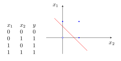
为什么感知器就可以解决线性问题呢？这是由它的传递函数决定的。这里以两个输入分量 x1 和 x2 组成的二维空间为例，此时节点 j 的输出为

所以，方程

确定的直线就是二维输入样本空间上的一条分界线。对于三维及更高维数的推导过程可以参考其他的Tutorials。

如果要让它来处理非线性的问题，单层感知器网就无能为力了。例如下面的“异或”，就无法用一条直线来分割开来，因此单层感知器网就没办法实现“异或”的功能。

使用Python 实现感知器学习算法

Perceptron.py

import numpy as np
#eta是学习率  n_iter是迭代次数
#errors_是每个阶段的错误数
#w_是权重吧
class Percetron(object):
    def __init__(self,eta=0.01,n_iter=10):
        self.eta=eta
        self.n_iter=n_iter
    def fit(self,X,y):
        self.w_=np.zeros(1+X.shape[1])#X的列数+1
        self.errors_=[]
        for _ in range(self.n_iter):#迭代次数
            errors=0
            for xi,target in zip(X,y):#将X,y组成
                update=self.eta*(target-self.predict(xi))#预测目标和实际目标是否相同
                self.w_[1:]+=update*xi#更新
                self.w_[0]+=update#更新b
                errors+=int(update != 0.0)#记录这次迭代的错误数
            self.errors_.append(errors)
        return  self#关键返回参数W
    def net_input(self,X):#输入X,输出结果
        return np.dot(X,self.w_[1:])+self.w_[0]
    def predict(self,X):
        return np.where(self.net_input(X)>=0.0,1,-1)#如果结果大于等于0，返回1，否则返回0

main.py

import pandas as pd
import matplotlib.pyplot as plt
import numpy as np
import Percetron as P
from matplotlib.colors import ListedColormap


def plot_decision_regions(X,y,classifier,resolution=0.02):#绘制决策边界
    markers=('s','x','o','^','v')#标记
    colors=('red','blue','lightgreen','gray','cyan')#颜色
    cmap=ListedColormap(colors[:len(np.unique(y))])#定义一些颜色和标记符号，并通过颜色列表生成了颜色示例图
    x1_min,x1_max=X[:,0].min()-1,X[:,0].max()+1#对最大值和最小值做出限定
    x2_min,x2_max=X[:,1].min()-1,X[:,1].max()+1
    xx1,xx2=np.meshgrid(np.arange(x1_min,x1_max,resolution),np.arange(x2_min,x2_max,resolution))
    Z=classifier.predict(np.array([xx1.ravel(),xx2.ravel()]).T)
    z=Z.reshape(xx1.shape)
    plt.xlim(xx1.min(),xx1.max())#x轴范围
    plt.ylim(xx2.min(),xx2.max())#y轴范围
    for idx,c1 in enumerate(np.unique(y)):
        plt.scatter(x=X[y==c1,0],y=X[y==c1,1],alpha=0.8,c=cmap(idx),marker=markers[idx],label=c1)






if __name__ == "__main__":
    df = pd.read_csv('https://archive.ics.uci.edu/ml/machine-learning-databases/iris/iris.data', header=None)
    df.tail()  # 用于显示数据的最后五行以确保加载成功
    y=df.iloc[0:100,4].values#此时y是类别名称
    y=np.where(y=='Iris-setosa',-1,1)#若是这个名称则为-1，不是则为1
    X=df.iloc[0:100,[0,2]].values#从表中获得X

    plt.scatter(X[:50,0],X[:50,1],color='red',marker='o',label='setosa')
    plt.scatter(X[50:100,0],X[50:100,1],color='blue',marker='x',label='versicolor')
    plt.xlabel('petal length')
    plt.ylabel('sepal length')
    plt.legend(loc='upper left')
    plt.show()

    ppn=P.Percetron(eta=0.1,n_iter=10)#初始化感知器
    ppn.fit(X,y)#拟合感知器
    plt.plot(range(1,len(ppn.errors_)+1),ppn.errors_,marker='o')#横坐标从1到len(errors_),纵坐标为errors_，
    plt.xlabel('Epochs')
    plt.ylabel('Number of misclassifications')
    plt.show()


    plot_decision_regions(X,y,classifier=ppn)
    plt.xlabel('sepal length [cm]')
    plt.ylabel('petal length [cm]')
    plt.legend(loc='upper left')
    plt.show()

自适应线性神经元及其学习的收敛性

在之前的文章感知机中提到过，感知机分类器是一个非常好的二分类分类器。

但是感知机分类器仍然存在两个比较明显的缺陷：

1. 感知机模型只能针对线性可分的数据集，对于非线性可分的数据集，无能为力
2. 当两个类可由线性超平面分离时，感知器学习规则收敛，但当类无法由线性分类器完美分离

为了解决感知机的这两个主要的缺陷，就有了现在要讲的自适应线性神经元

在之前的感知机中，感知机的激活函数是阶跃函数，这里改为线性激活函数（linear activation function）,一般来说，为了方便，可以直接取：

感知机框架和自适应线性神经元框架对比，注意，自适应线性神经元框架比感知机框架多了一个量化器（quantizer），其主要作用是得到样本的类别。

梯度下降法（Gradient Descent）

相对于阶跃函数而言，线性函数有一个明显的优点：函数是可微（differentiable）的。这就使得我们可以直接在这个函数上定义损失函数 J(W)（cost function），并对其进行优化。这里定义损失函数J(W)为平方损失误差和（SSE： sum of squared errors），这里假设训练样本集合的大小为n ：

AdalineGD.py

import numpy as np
import matplotlib.pyplot as plt
import pandas as pd



class AdalineGD(object):
    def __init__(self,eta=0.01,n_iter=50):
        self.eta=eta
        self.n_iter=n_iter
    def fit(self,X,y):
        self.w_=np.zeros(1+X.shape[1])
        self.cost_=[]
        for i in range(self.n_iter):
            output=self.net_input(X)
            errors=(y-output)
            self.w_[1:]+=self.eta*X.T.dot(errors)
            self.w_[0]+=self.eta*errors.sum()
            cost=(errors**2).sum()/2
            self.cost_.append(cost)
        return self
    def net_input(self,X):
        return np.dot(X,self.w_[1:])+self.w_[0]
    def activation(self,X):
        return self.net_input(X)
    def predict(self,X):
        return np.where(self.activation(X)>=0,1,-1)
if __name__ == "__main__":
    df = pd.read_csv('https://archive.ics.uci.edu/ml/machine-learning-databases/iris/iris.data', header=None)
    df.tail()  # 用于显示数据的最后五行以确保加载成功
    y = df.iloc[0:100, 4].values  # 此时y是类别名称
    y = np.where(y == 'Iris-setosa', -1, 1)  # 若是这个名称则为-1，不是则为1
    X = df.iloc[0:100, [0, 2]].values  # 从表中获得X
    fig,ax=plt.subplots(nrows=1,ncols=2,figsize=(8,4))
    ada1=AdalineGD(n_iter=10,eta=0.01).fit(X,y)
    ax[0].plot(range(1,len(ada1.cost_)+1),np.log10(ada1.cost_),marker='o')
    ax[0].set_xlabel('Epochs')
    ax[0].set_ylabel('log(Sum-squared-error)')
    ax[0].set_title('Adaline-Learning rate 0.01')
    ada2=AdalineGD(n_iter=10,eta=0.0001).fit(X,y)
    ax[1].plot(range(1,len(ada2.cost_)+1),ada2.cost_,marker='o')
    ax[1].set_xlabel('Epochs')
    ax[1].set_ylabel('Sum-squared-error')
    ax[1].set_title('Adaline-Learning rate 0.0001')
    plt.show()