P73 卷积神经网络识别手写数字

https://www.bilibili.com/video/BV184411Q7Ng?p=73

 

 数据集介绍：

 

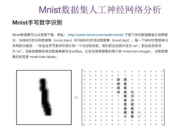
 1.设计占位符：

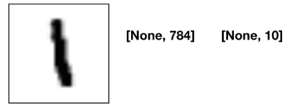
 注解：

• [None, 784] 样本数据量未知。[None, 10] 每个样本都有10个类别的概率。

2.设计网络结构：

 

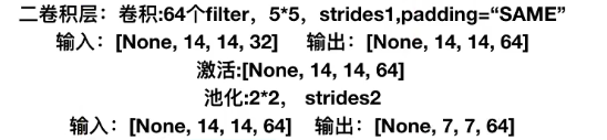
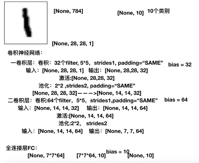
注解：

• 最后一层全连接层，[7,7,64]要变成一个二维的矩阵，[7*7*64]，就是说用这么多的特征数量和10个神经元进行全连接。再经过sigmoid函数的作用，变成10个概率值。

"""
用单层神经网络实现手写数字识别


def conv2d(input, filter, strides, padding, use_cudnn_on_gpu=True, data_format="NHWC", dilations=[1, 1, 1, 1], name=None):
  Computes a 2-D convolution given 4-D `input` and `filter` tensors.
    参数说明：
  Given an input tensor of shape `[batch, in_height, in_width, in_channels]`
  and a filter / kernel tensor of shape
  `[filter_height, filter_width, in_channels, out_channels]`, this op
  performs the following:

  1. Flattens the filter to a 2-D matrix with shape
     `[filter_height * filter_width * in_channels, output_channels]`.
  2. Extracts image patches from the input tensor to form a *virtual*
     tensor of shape `[batch, out_height, out_width,
     filter_height * filter_width * in_channels]`.
  3. For each patch, right-multiplies the filter matrix and the image patch
     vector.



"""
import tensorflow as tf
from tensorflow.examples.tutorials.mnist import input_data
#FLAGS=tf.app.flags.FlAGS
#tf.app.flags.DEFINE_integer("is_train",1,"指定程序是预测还是训练")
#is_train=1 #is_train的值设为1,代表是训练
is_train=0 #is_train的值设为0,代表是训练之后的预测
def full_connected():
    mnist=input_data.read_data_sets("./data/mnist/input_data/",one_hot=True)
    #建立数据的占位符，　x [None,784] y_true [None,10]
    with tf.variable_scope("data"):
        x=tf.placeholder(tf.float32,[None,784])
        y_true=tf.placeholder(tf.int32,[None,10])
    #2、建立一个全连接层的神经网络w [784,10] b [10]
    with tf.variable_scope("fc_model"):
        # 随机初始化权重和偏置
        weight=tf.Variable(tf.random_normal([784,10],mean=0.0,stddev=1.0,name='w'))
        bias=tf.Variable(tf.constant(0.0,shape=[10]))
        #预测None个样本的输出结果[None, 784]*[784,10]+[10]=[None,10]
        y_predict=tf.matmul(x,weight)+bias
    #3、求出所有样本的损失
    with tf.variable_scope("soft_cross"):
        #求平均的交叉熵损失
        loss=tf.reduce_mean(tf.nn.softmax_cross_entropy_with_logits(labels=y_true,logits=y_predict))
     #4、梯度下降求损失
    with tf.variable_scope("optimizer"):
        train_op=tf.train.GradientDescentOptimizer(0.1).minimize(loss)
    #5、计算准确率
    with tf.variable_scope("acc"):
        equal_list=tf.equal(tf.argmax(y_true,1),tf.argmax(y_predict,1))
        #equal_list is None个样本　　[1,0,1,1,0,0,0,1,1,0...]
        accuracy=tf.reduce_mean(tf.cast(equal_list,tf.float32))
    # 收集变量，单个数字值的收集
    tf.summary.scalar("losses",loss)#收集损失
    tf.summary.scalar("acc",accuracy)#收集准确率
    # 高维度变量收集
    tf.summary.histogram("weightes",weight)
    tf.summary.histogram("biases",bias)


    # 定义一个初始化的变量op
    init_op=tf.global_variables_initializer()
    # 定义一个合并变量的op
    merged=tf.summary.merge_all()

    #　创建一个saver
    saver=tf.train.Saver()


    #开启会话去训练
    with tf.Session() as sess:
        #初始化变量
        sess.run(init_op)

        #建立events文件，然后写入
        filewriter=tf.summary.FileWriter("./tmp/summary/test/",graph=sess.graph)

        if is_train==1:


            #迭代步数去训练，更新参数进行预测
            for i in range(2000):
                #取出样本的特征值和目标值
                mnist_x,mnist_y=mnist.train.next_batch(50)
                #运行train_op训练
                sess.run(train_op,feed_dict={x:mnist_x,y_true:mnist_y})



                # 写入每步训练的值
                summary=sess.run(merged,feed_dict={x:mnist_x,y_true:mnist_y})

                filewriter.add_summary(summary,i)

                print("训练第%d步，准确率为:%f"%(i,sess.run(accuracy,feed_dict={x:mnist_x,y_true:mnist_y})))

            #保存模型
            saver.save(sess,"./tmp/ckpt/fc_model")
        else:
            # 加载模型，主要是加载训练之后保存在模型中的weight和bias
            saver.restore(sess,"./tmp/ckpt/fc_model")
            # 如果是0，做预测
            for i in range(100):
                # 每次测试一张图片
                x_test,y_test=mnist.test.next_batch(1)
                print("第%d张图片，手写数字图片目标是：%d,预测结果是：%d"%(
                    i,
                    tf.argmax(y_test,1).eval(),
                    tf.argmax(sess.run(y_predict,feed_dict={x:x_test,y_true:y_test}),1).eval()
                ))

    return None



def weight_variables(shape):
    """
    自定义一个随机初始化权重的函数
    因为w是要迭代更新的，所以它要定义成一个tf的变量
    """
    w=tf.Variable(tf.random_normal(shape=shape,mean=0.0,stddev=1.0))
    return w


def bias_variables(shape):
    """
    自定义一个随机初始化偏置的函数
    """
    b=tf.Variable(tf.constant(0.0,shape=shape))
    return b




def model():
    """
    自定义一个卷积模型
    :return:
    """
    """
    1、准备数据的占位符
    """
    # 1、准备数据的占位符，　x [None,784] y_true [None,10]
    with tf.variable_scope("data"):
        x = tf.placeholder(tf.float32, [None, 784])
        y_true = tf.placeholder(tf.int32, [None, 10])
    """
    2、卷积层１，卷积:核->5*5*1,strides=1,padding="SAME"
    激活,tf.nn.relu、池化
    """
    with tf.variable_scope("conv1"):
        #要有一些随机初始化的权重w和偏置bias
        # 随机初始化权重
        w_conv1=weight_variables([5,5,1,32])

        # 随机初始化bias,有多少个filter,就有多少个bias
        b_conv1=bias_variables([32])

        #因为tf.nn.conv2d()的第一个参数是：[batch, in_height, in_width, in_channels]
        #所以需要把输入数据改成张量 [None,784]->[None,28,28,1]
        x_reshape=tf.reshape(x,[-1,28,28,1]) #当不知道有多少样本的时候，此处不能填写None,要填写-1


        # 卷积：[None,28,28,1]->[None,28,28,32]
        conv1=tf.nn.conv2d(x_reshape,w_conv1,strides=[1,1,1,1],padding="SAME")+b_conv1
        x_relu1=tf.nn.relu(conv1)# 卷积后使之经过激活函数

        # 池化 pooling,2*2,strides=2　[None,28,28,32]->[None,14,14,32]
        x_pool1=tf.nn.max_pool(x_relu1,ksize=[1,2,2,1],strides=[1,2,2,1],padding="SAME")

    """
    2、卷积层2，卷积核->5*5*32,filter=64,strides=1,padding="SAME"
    激活,tf.nn.relu、池化
    注意：每一张图像的通道数此时变成了32
    卷积核此时应是：5*5*32，因为一个人要观察32张图，共有64个人观察
    
    """
    with tf.variable_scope("conv2"):
        # 要有一些随机初始化的权重w和偏置bias
        # 随机初始化权重
        w_conv2 = weight_variables([5, 5, 32, 64])

        # 随机初始化bias,有多少个filter,就有多少个bias
        b_conv2 = bias_variables([64])

        # 卷积，激活，池化计算：[None,14,14,32]->[None,14,14,64]
        conv2 = tf.nn.conv2d(x_pool1, w_conv2, strides=[1, 1, 1, 1], padding="SAME") + b_conv2
        x_relu2 = tf.nn.relu(conv2)  # 卷积后使之经过激活函数

        # 池化 pooling,2*2,strides=2　[None,14,14,64]->[None,7,7,64]
        x_pool2 = tf.nn.max_pool(x_relu2, ksize=[1, 2, 2, 1], strides=[1,2,2,1], padding="SAME")

    """
    4、全连接层
    [None,7,7,64]->[None,7*7*64]*[7*7*64(权重数),10]+[10]=[None,10]
    """
    with tf.variable_scope("full_connected"):

        #随机初始化权重和偏置
        w_fc=weight_variables([7*7*64,10])
        b_fc=bias_variables([10])

        #进行矩阵运算得出每个样本的10个结果
        # 进行矩阵运算之前，修改形状：4维张量到2维矩阵
        # [None,7,7,64]->[None,7*7*64]
        x_pool2_reshape = tf.reshape(x_pool2, [-1, 7*7*64]) #-1代表不知道多少个样本，每个样本都是7*7*64个特征
        y_predict=tf.matmul(x_pool2_reshape,w_fc)+b_fc

    return x,y_true,y_predict

def conv_fc():
    # 获取真实的数据
    mnist=input_data.read_data_sets("./data/mnist/input_data/",one_hot=True)
    x,y_true,y_predict=model()

    #进行交叉熵损失的计算
    #求出所有样本的损失，然后求平均值
    #3、求出所有样本的损失
    with tf.variable_scope("soft_cross"):
        #求平均的交叉熵损失
        loss=tf.reduce_mean(tf.nn.softmax_cross_entropy_with_logits(labels=y_true,logits=y_predict))


    #4、梯度下降求损失
    with tf.variable_scope("optimizer"):
        train_op=tf.train.GradientDescentOptimizer(0.1).minimize(loss)
    #5、计算准确率
    with tf.variable_scope("acc"):
        equal_list=tf.equal(tf.argmax(y_true,1),tf.argmax(y_predict,1))
        #equal_list is None个样本　　[1,0,1,1,0,0,0,1,1,0...]
        accuracy=tf.reduce_mean(tf.cast(equal_list,tf.float32))


    # 定义一个初始化的变量op
    init_op=tf.global_variables_initializer()

    #开启会话运行程序
    with tf.Session() as sess:
        sess.run(init_op) #进行变量初始化

        #循环去训练


        # 迭代步数去训练，更新参数进行预测
        for i in range(1000):
            # 取出样本的特征值和目标值
            mnist_x, mnist_y = mnist.train.next_batch(50)
            # 运行train_op训练
            sess.run(train_op, feed_dict={ x: mnist_x, y_true: mnist_y})

            print("训练第%d步，准确率为:%f"%(i,sess.run(accuracy,feed_dict={x:mnist_x,y_true:mnist_y})))





if __name__ == '__main__':
    conv_fc()

运行结果：

训练第0步，准确率为:0.200000
训练第1步，准确率为:0.200000
训练第2步，准确率为:0.160000
训练第3步，准确率为:0.060000
训练第4步，准确率为:0.120000
训练第5步，准确率为:0.100000
训练第6步，准确率为:0.200000
训练第7步，准确率为:0.140000

.

.

.

训练第995步，准确率为:0.100000
训练第996步，准确率为:0.100000
训练第997步，准确率为:0.080000
训练第998步，准确率为:0.140000
训练第999步，准确率为:0.120000

这样收敛过慢的结果，原因考虑学习率太大。

"""
用单层神经网络实现手写数字识别


def conv2d(input, filter, strides, padding, use_cudnn_on_gpu=True, data_format="NHWC", dilations=[1, 1, 1, 1], name=None):
  Computes a 2-D convolution given 4-D `input` and `filter` tensors.
    参数说明：
  Given an input tensor of shape `[batch, in_height, in_width, in_channels]`
  and a filter / kernel tensor of shape
  `[filter_height, filter_width, in_channels, out_channels]`, this op
  performs the following:

  1. Flattens the filter to a 2-D matrix with shape
     `[filter_height * filter_width * in_channels, output_channels]`.
  2. Extracts image patches from the input tensor to form a *virtual*
     tensor of shape `[batch, out_height, out_width,
     filter_height * filter_width * in_channels]`.
  3. For each patch, right-multiplies the filter matrix and the image patch
     vector.



"""
import tensorflow as tf
from tensorflow.examples.tutorials.mnist import input_data
#FLAGS=tf.app.flags.FlAGS
#tf.app.flags.DEFINE_integer("is_train",1,"指定程序是预测还是训练")
#is_train=1 #is_train的值设为1,代表是训练
is_train=0 #is_train的值设为0,代表是训练之后的预测
def full_connected():
    mnist=input_data.read_data_sets("./data/mnist/input_data/",one_hot=True)
    #建立数据的占位符，　x [None,784] y_true [None,10]
    with tf.variable_scope("data"):
        x=tf.placeholder(tf.float32,[None,784])
        y_true=tf.placeholder(tf.int32,[None,10])
    #2、建立一个全连接层的神经网络w [784,10] b [10]
    with tf.variable_scope("fc_model"):
        # 随机初始化权重和偏置
        weight=tf.Variable(tf.random_normal([784,10],mean=0.0,stddev=1.0,name='w'))
        bias=tf.Variable(tf.constant(0.0,shape=[10]))
        #预测None个样本的输出结果[None, 784]*[784,10]+[10]=[None,10]
        y_predict=tf.matmul(x,weight)+bias
    #3、求出所有样本的损失
    with tf.variable_scope("soft_cross"):
        #求平均的交叉熵损失
        loss=tf.reduce_mean(tf.nn.softmax_cross_entropy_with_logits(labels=y_true,logits=y_predict))
     #4、梯度下降求损失
    with tf.variable_scope("optimizer"):
        train_op=tf.train.GradientDescentOptimizer(0.1).minimize(loss)
    #5、计算准确率
    with tf.variable_scope("acc"):
        equal_list=tf.equal(tf.argmax(y_true,1),tf.argmax(y_predict,1))
        #equal_list is None个样本　　[1,0,1,1,0,0,0,1,1,0...]
        accuracy=tf.reduce_mean(tf.cast(equal_list,tf.float32))
    # 收集变量，单个数字值的收集
    tf.summary.scalar("losses",loss)#收集损失
    tf.summary.scalar("acc",accuracy)#收集准确率
    # 高维度变量收集
    tf.summary.histogram("weightes",weight)
    tf.summary.histogram("biases",bias)


    # 定义一个初始化的变量op
    init_op=tf.global_variables_initializer()
    # 定义一个合并变量的op
    merged=tf.summary.merge_all()

    #　创建一个saver
    saver=tf.train.Saver()


    #开启会话去训练
    with tf.Session() as sess:
        #初始化变量
        sess.run(init_op)

        #建立events文件，然后写入
        filewriter=tf.summary.FileWriter("./tmp/summary/test/",graph=sess.graph)

        if is_train==1:


            #迭代步数去训练，更新参数进行预测
            for i in range(2000):
                #取出样本的特征值和目标值
                mnist_x,mnist_y=mnist.train.next_batch(50)
                #运行train_op训练
                sess.run(train_op,feed_dict={x:mnist_x,y_true:mnist_y})



                # 写入每步训练的值
                summary=sess.run(merged,feed_dict={x:mnist_x,y_true:mnist_y})

                filewriter.add_summary(summary,i)

                print("训练第%d步，准确率为:%f"%(i,sess.run(accuracy,feed_dict={x:mnist_x,y_true:mnist_y})))

            #保存模型
            saver.save(sess,"./tmp/ckpt/fc_model")
        else:
            # 加载模型，主要是加载训练之后保存在模型中的weight和bias
            saver.restore(sess,"./tmp/ckpt/fc_model")
            # 如果是0，做预测
            for i in range(100):
                # 每次测试一张图片
                x_test,y_test=mnist.test.next_batch(1)
                print("第%d张图片，手写数字图片目标是：%d,预测结果是：%d"%(
                    i,
                    tf.argmax(y_test,1).eval(),
                    tf.argmax(sess.run(y_predict,feed_dict={x:x_test,y_true:y_test}),1).eval()
                ))

    return None



def weight_variables(shape):
    """
    自定义一个随机初始化权重的函数
    因为w是要迭代更新的，所以它要定义成一个tf的变量
    """
    w=tf.Variable(tf.random_normal(shape=shape,mean=0.0,stddev=1.0))
    return w


def bias_variables(shape):
    """
    自定义一个随机初始化偏置的函数
    """
    b=tf.Variable(tf.constant(0.0,shape=shape))
    return b




def model():
    """
    自定义一个卷积模型
    :return:
    """
    """
    1、准备数据的占位符
    """
    # 1、准备数据的占位符，　x [None,784] y_true [None,10]
    with tf.variable_scope("data"):
        x = tf.placeholder(tf.float32, [None, 784])
        y_true = tf.placeholder(tf.int32, [None, 10])
    """
    2、卷积层１，卷积:核->5*5*1,strides=1,padding="SAME"
    激活,tf.nn.relu、池化
    """
    with tf.variable_scope("conv1"):
        #要有一些随机初始化的权重w和偏置bias
        # 随机初始化权重
        w_conv1=weight_variables([5,5,1,32])

        # 随机初始化bias,有多少个filter,就有多少个bias
        b_conv1=bias_variables([32])

        #因为tf.nn.conv2d()的第一个参数是：[batch, in_height, in_width, in_channels]
        #所以需要把输入数据改成张量 [None,784]->[None,28,28,1]
        x_reshape=tf.reshape(x,[-1,28,28,1]) #当不知道有多少样本的时候，此处不能填写None,要填写-1


        # 卷积：[None,28,28,1]->[None,28,28,32]
        conv1=tf.nn.conv2d(x_reshape,w_conv1,strides=[1,1,1,1],padding="SAME")+b_conv1
        x_relu1=tf.nn.relu(conv1)# 卷积后使之经过激活函数

        # 池化 pooling,2*2,strides=2　[None,28,28,32]->[None,14,14,32]
        x_pool1=tf.nn.max_pool(x_relu1,ksize=[1,2,2,1],strides=[1,2,2,1],padding="SAME")

    """
    2、卷积层2，卷积核->5*5*32,filter=64,strides=1,padding="SAME"
    激活,tf.nn.relu、池化
    注意：每一张图像的通道数此时变成了32
    卷积核此时应是：5*5*32，因为一个人要观察32张图，共有64个人观察
    
    """
    with tf.variable_scope("conv2"):
        # 要有一些随机初始化的权重w和偏置bias
        # 随机初始化权重
        w_conv2 = weight_variables([5, 5, 32, 64])

        # 随机初始化bias,有多少个filter,就有多少个bias
        b_conv2 = bias_variables([64])

        # 卷积，激活，池化计算：[None,14,14,32]->[None,14,14,64]
        conv2 = tf.nn.conv2d(x_pool1, w_conv2, strides=[1, 1, 1, 1], padding="SAME") + b_conv2
        x_relu2 = tf.nn.relu(conv2)  # 卷积后使之经过激活函数

        # 池化 pooling,2*2,strides=2　[None,14,14,64]->[None,7,7,64]
        x_pool2 = tf.nn.max_pool(x_relu2, ksize=[1, 2, 2, 1], strides=[1,2,2,1], padding="SAME")

    """
    4、全连接层
    [None,7,7,64]->[None,7*7*64]*[7*7*64(权重数),10]+[10]=[None,10]
    """
    with tf.variable_scope("full_connected"):

        #随机初始化权重和偏置
        w_fc=weight_variables([7*7*64,10])
        b_fc=bias_variables([10])

        #进行矩阵运算得出每个样本的10个结果
        # 进行矩阵运算之前，修改形状：4维张量到2维矩阵
        # [None,7,7,64]->[None,7*7*64]
        x_pool2_reshape = tf.reshape(x_pool2, [-1, 7*7*64]) #-1代表不知道多少个样本，每个样本都是7*7*64个特征
        y_predict=tf.matmul(x_pool2_reshape,w_fc)+b_fc

    return x,y_true,y_predict

def conv_fc():
    # 获取真实的数据
    mnist=input_data.read_data_sets("./data/mnist/input_data/",one_hot=True)
    x,y_true,y_predict=model()

    #进行交叉熵损失的计算
    #求出所有样本的损失，然后求平均值
    #3、求出所有样本的损失
    with tf.variable_scope("soft_cross"):
        #求平均的交叉熵损失
        loss=tf.reduce_mean(tf.nn.softmax_cross_entropy_with_logits(labels=y_true,logits=y_predict))


    #4、梯度下降求损失
    with tf.variable_scope("optimizer"):
        train_op=tf.train.GradientDescentOptimizer(0.0001).minimize(loss)
    #5、计算准确率
    with tf.variable_scope("acc"):
        equal_list=tf.equal(tf.argmax(y_true,1),tf.argmax(y_predict,1))
        #equal_list is None个样本　　[1,0,1,1,0,0,0,1,1,0...]
        accuracy=tf.reduce_mean(tf.cast(equal_list,tf.float32))


    # 定义一个初始化的变量op
    init_op=tf.global_variables_initializer()

    #开启会话运行程序
    with tf.Session() as sess:
        sess.run(init_op) #进行变量初始化

        #循环去训练


        # 迭代步数去训练，更新参数进行预测
        for i in range(2000):
            # 取出样本的特征值和目标值
            mnist_x, mnist_y = mnist.train.next_batch(50)
            # 运行train_op训练
            sess.run(train_op, feed_dict={ x: mnist_x, y_true: mnist_y})

            print("训练第%d步，准确率为:%f"%(i,sess.run(accuracy,feed_dict={x:mnist_x,y_true:mnist_y})))





if __name__ == '__main__':
    conv_fc()

学习率改成了0.0001,循环步数改成了2000次的运行结果是：

训练第0步，准确率为:0.080000
训练第1步，准确率为:0.160000
训练第2步，准确率为:0.100000
训练第3步，准确率为:0.180000
训练第4步，准确率为:0.180000
训练第5步，准确率为:0.120000

.

.

.

训练第1995步，准确率为:0.780000
训练第1996步，准确率为:0.800000
训练第1997步，准确率为:0.820000
训练第1998步，准确率为:0.780000
训练第1999步，准确率为:0.820000

注解：

• 准确率得到了明显的提升。
• 最后的一个全连接层的激活函数是softmax.

常见的网络结构：

 

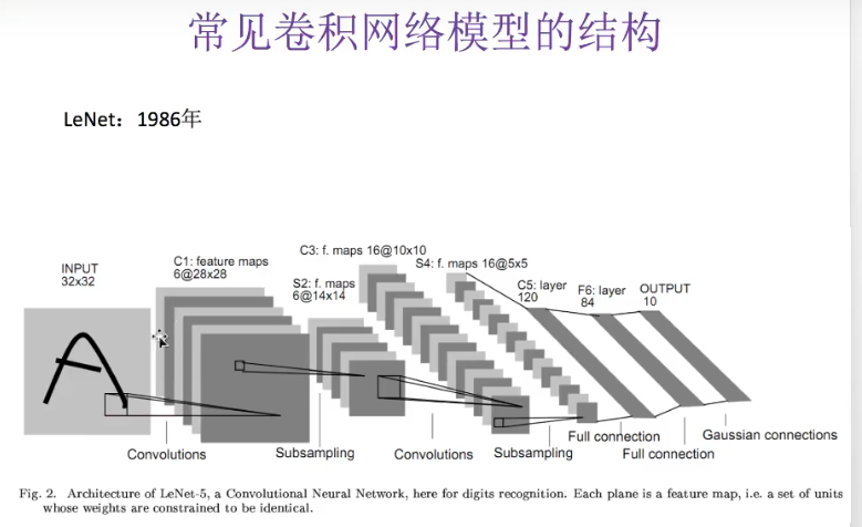
 注解：

• 杨乐昆写的。

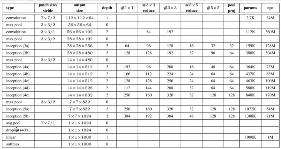
 注解：

• 参数数量6千万级别，一般的机器跑这个网络是跑不动的。

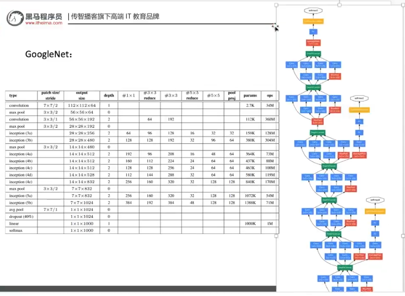
 注解：

• 这个是googlenet网络。
• inception是特定的网络结构。
• 加入dropout是因为参数太多了，需要随机丢失一些，以减少计算量，最主要的目的还是降低过拟合。

 

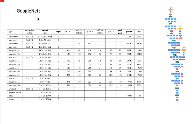
注解：

•  tensorflow的库里面已经实现了googlenet的inception结构。
• 如果图片像素数量比较多，可以考虑使用inception结构。