import torch
import torch.nn.functional as F
import matplotlib.pyplot as plt

# torch.manual_seed(1)    # reproducible

x = torch.unsqueeze(torch.linspace(-1, 1, 100), dim=1)  # 将1维数据转换成2维数据,torch不能处理1维数据。x data (tensor), shape=(100, 1)
y = x.pow(2) + 0.2*torch.rand(x.size())                 # noisy y data (tensor), shape=(100, 1)

# torch can only train on Variable, so convert them to Variable
# The code below is deprecated in Pytorch 0.4. Now, autograd directly supports tensors
# x, y = Variable(x), Variable(y)

# plt.scatter(x.data.numpy(), y.data.numpy())
# plt.show()  # 有噪音的抛物线图


class Net(torch.nn.Module):  # 输入特征,线性处理进入隐藏层的数据,线性处理进入输出层的数据
    def __init__(self, n_feature, n_hidden, n_output):
        super(Net, self).__init__()
        self.hidden = torch.nn.Linear(n_feature, n_hidden)   # hidden layer
        self.predict = torch.nn.Linear(n_hidden, n_output)   # output layer

    def forward(self, x):   # 激活一下进入隐藏层的数据
        x = F.relu(self.hidden(x))      # activation function for hidden layer
        x = self.predict(x)             # linear output
        return x

net = Net(n_feature=1, n_hidden=10, n_output=1)     # define the network 的大小
print(net)  # 显示网络结构 net architecture
> Net(
>   (hidden): Linear(in_features=1, out_features=10, bias=True)
>   (predict): Linear(in_features=10, out_features=1, bias=True)
> )
optimizer = torch.optim.SGD(net.parameters(), lr=0.2) # 设置优化器优化网络(优化参数,学习率)
loss_func = torch.nn.MSELoss() # 均方差处理回归问题 this is for regression mean squared loss
# plt.ion() # something about plotting
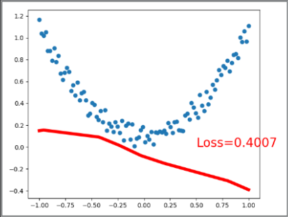
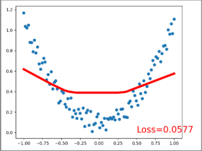
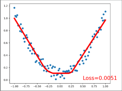
for t in range(200): # 训练的过程
prediction = net(x) # input x and predict based on x
loss = loss_func(prediction, y) # 计算预测值和真实值的误差,预测值在前面,顺序不同可能影响结算结果 must be (1. nn output, 2. target)
optimizer.zero_grad() # 梯度重置为零 clear gradients for next train
loss.backward() # 开始这次的反向传递,计算梯度 backpropagation, compute gradients
optimizer.step() # 使用优化器优化梯度,apply gradients
if t % 5 == 0:
# 可视化显示训练过程 plot and show learning process
plt.cla()
plt.scatter(x.data.numpy(), y.data.numpy())
plt.plot(x.data.numpy(), prediction.data.numpy(), 'r-', lw=5)
plt.text(0.5, 0, 'Loss=%.4f' % loss.data.numpy(), fontdict={'size': 20, 'color': 'red'})
plt.pause(0.1)
# plt.ioff()
plt.show()
END