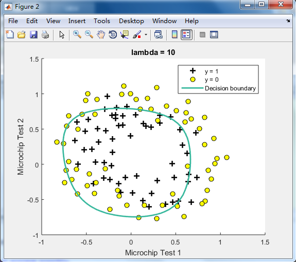
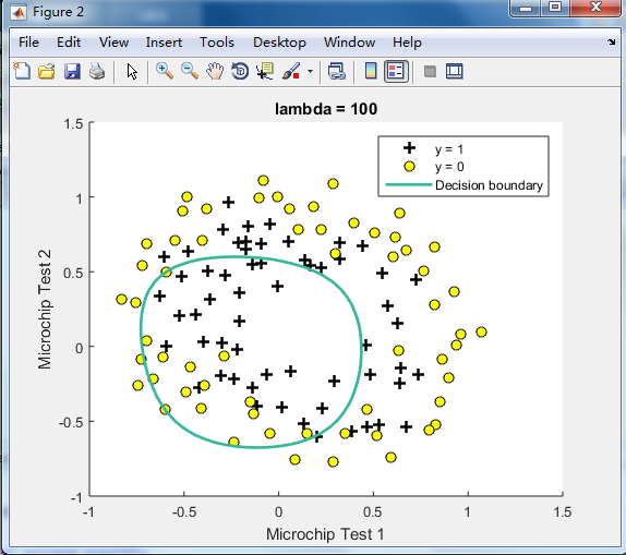
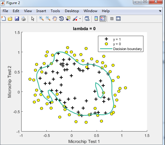
不同的λ(0,1,10,100)值对regularization的影响 预测新的值和计算模型的精度
%% ============= Part 2: Regularization and Accuracies =============
% Optional Exercise:
% In this part, you will get to try different values of lambda and
% see how regularization affects the decision coundart
%
% Try the following values of lambda (0, 1, 10, 100).
%
% How does the decision boundary change when you vary lambda? How does
% the training set accuracy vary?
%
% Initialize fitting parameters
initial_theta = zeros(size(X, 2), 1);
% Set regularization parameter lambda to 1 (you should vary this)
lambda = 1; %在这里设置λ=(0,1,10,100)
由下图可见,lambda=1时的效果最好,
λ=0时No regularization(overfitting);
λ=100时会too much regularization(underfitting),
% Set Options
options = optimset('GradObj', 'on', 'MaxIter', 400); %计算gradient,迭代的次数为400次
% Optimize
[theta, J, exit_flag] = ...
fminunc(@(t)(costFunctionReg(t, X, y, lambda)), initial_theta, options);
% Plot Boundary
plotDecisionBoundary(theta, X, y); %X已经mapFeature过了
hold on;
title(sprintf('lambda = %g', lambda)) % 会在%e和%f中自动选择一种格式,且无后缀0。
% Labels and Legend
xlabel('Microchip Test 1')
ylabel('Microchip Test 2')
legend('y = 1', 'y = 0', 'Decision boundary')
hold off;
% Compute accuracy on our training set
p = predict(theta, X);
fprintf('Train Accuracy: %f ', mean(double(p == y)) * 100);
plotDecisionBoundary.m文件
function plotDecisionBoundary(theta, X, y)
%PLOTDECISIONBOUNDARY Plots the data points X and y into a new figure with
%the decision boundary defined by theta
% PLOTDECISIONBOUNDARY(theta, X,y) plots the data points with + for the
% positive examples and o for the negative examples. X is assumed to be
% a either
% 1) Mx3 matrix, where the first column is an all-ones column for the
% intercept.
% 2) MxN, N>3 matrix, where the first column is all-ones
% Plot Data
plotData(X(:,2:3), y);
hold on
if size(X, 2) <= 3
% Only need 2 points to define a line, so choose two endpoints
plot_x = [min(X(:,2))-2, max(X(:,2))+2];
% Calculate the decision boundary line
plot_y = (-1./theta(3)).*(theta(2).*plot_x + theta(1));
% Plot, and adjust axes for better viewing
plot(plot_x, plot_y)
% Legend, specific for the exercise
legend('Admitted', 'Not admitted', 'Decision Boundary')
axis([30, 100, 30, 100])
else %X已经mapFeature过了(有28个features),调用这部分的程序
% Here is the grid range
u = linspace(-1, 1.5, 50);
v = linspace(-1, 1.5, 50);
z = zeros(length(u), length(v));
% Evaluate z = theta*x over the grid
for i = 1:length(u)
for j = 1:length(v)
z(i,j) = mapFeature(u(i), v(j))*theta;
end
end
z = z'; % important to transpose z before calling contour
% Plot z = 0
% Notice you need to specify the range [0, 0]
contour(u, v, z, [0, 0], 'LineWidth', 2) %画等值线.contour(X,Y,Z,[v v]) to draw contours for the single level v.
end %if size(X, 2) <= 3 else的end
hold off
end
predict.m文件
function p = predict(theta, X)
%PREDICT Predict whether the label is 0 or 1 using learned logistic
%regression parameters theta
% p = PREDICT(theta, X) computes the predictions for X using a
% threshold at 0.5 (i.e., if sigmoid(theta'*x) >= 0.5, predict 1)
m = size(X, 1); % Number of training examples
% You need to return the following variables correctly
p = zeros(m, 1);
% ====================== YOUR CODE HERE ======================
% Instructions: Complete the following code to make predictions using
% your learned logistic regression parameters.
% You should set p to a vector of 0's and 1's
%
for i=1:m
if sigmoid(X(i,:) * theta) >=0.5
p(i) = 1;
else
p(i) = 0;
end
end
% =========================================================================
end


