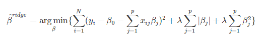
弹性网回归是lasso回归和岭回归的结合,其代价函数为:
若令 ,则
,则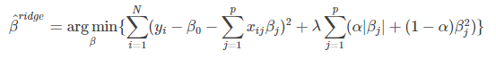
由此可知,弹性网的惩罚系数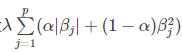 恰好为岭回归罚函数和Lasso罚函数的一个凸线性组合.当α=0时,弹性网回归即为岭回归;当 α=1时,弹性网回归即为Lasso回归.因此,弹性网回归兼有Lasso回归和岭回归的优点,既能达到变量选择的目的,又具有很好的群组效应。
上述解释摘自:https://blog.csdn.net/weixin_41500849/article/details/80447501
接下来是实现代码,代码来源: https://github.com/eriklindernoren/ML-From-Scratch
首先还是定义一个基类,各种线性回归都需要继承该基类:
class Regression(object):
    """ Base regression model. Models the relationship between a scalar dependent variable y and the independent
    variables X.
    Parameters:
    -----------
    n_iterations: float
        The number of training iterations the algorithm will tune the weights for.
    learning_rate: float
        The step length that will be used when updating the weights.
    """
    def __init__(self, n_iterations, learning_rate):
        self.n_iterations = n_iterations
        self.learning_rate = learning_rate

    def initialize_weights(self, n_features):
        """ Initialize weights randomly [-1/N, 1/N] """
        limit = 1 / math.sqrt(n_features)
        self.w = np.random.uniform(-limit, limit, (n_features, ))

    def fit(self, X, y):
        # Insert constant ones for bias weights
        X = np.insert(X, 0, 1, axis=1)
        self.training_errors = []
        self.initialize_weights(n_features=X.shape[1])

        # Do gradient descent for n_iterations
        for i in range(self.n_iterations):
            y_pred = X.dot(self.w)
            # Calculate l2 loss
            mse = np.mean(0.5 * (y - y_pred)**2 + self.regularization(self.w))
            self.training_errors.append(mse)
            # Gradient of l2 loss w.r.t w
            grad_w = -(y - y_pred).dot(X) + self.regularization.grad(self.w)
            # Update the weights
            self.w -= self.learning_rate * grad_w

    def predict(self, X):
        # Insert constant ones for bias weights
        X = np.insert(X, 0, 1, axis=1)
        y_pred = X.dot(self.w)
        return y_pred
然后是弹性网回归的核心:
class l1_l2_regularization():
    """ Regularization for Elastic Net Regression """
    def __init__(self, alpha, l1_ratio=0.5):
        self.alpha = alpha
        self.l1_ratio = l1_ratio

    def __call__(self, w):
        l1_contr = self.l1_ratio * np.linalg.norm(w)
        l2_contr = (1 - self.l1_ratio) * 0.5 * w.T.dot(w)
        return self.alpha * (l1_contr + l2_contr)

    def grad(self, w):
        l1_contr = self.l1_ratio * np.sign(w)
        l2_contr = (1 - self.l1_ratio) * w
        return self.alpha * (l1_contr + l2_contr)
接着是弹性网回归的代码:
class ElasticNet(Regression):
    """ Regression where a combination of l1 and l2 regularization are used. The
    ratio of their contributions are set with the 'l1_ratio' parameter.
    Parameters:
    -----------
    degree: int
        The degree of the polynomial that the independent variable X will be transformed to.
    reg_factor: float
        The factor that will determine the amount of regularization and feature
        shrinkage.
    l1_ration: float
        Weighs the contribution of l1 and l2 regularization.
    n_iterations: float
        The number of training iterations the algorithm will tune the weights for.
    learning_rate: float
        The step length that will be used when updating the weights.
    """
    def __init__(self, degree=1, reg_factor=0.05, l1_ratio=0.5, n_iterations=3000,
                learning_rate=0.01):
        self.degree = degree
        self.regularization = l1_l2_regularization(alpha=reg_factor, l1_ratio=l1_ratio)
        super(ElasticNet, self).__init__(n_iterations,
                                        learning_rate)

    def fit(self, X, y):
        X = normalize(polynomial_features(X, degree=self.degree))
        super(ElasticNet, self).fit(X, y)

    def predict(self, X):
        X = normalize(polynomial_features(X, degree=self.degree))
        return super(ElasticNet, self).predict(X)
其中涉及到的一些函数可参考:https://www.cnblogs.com/xiximayou/p/12802868.html
最后是运行主函数:
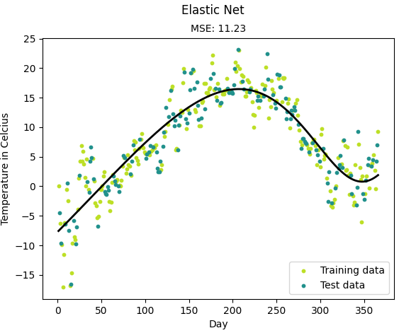
from __future__ import print_function
import matplotlib.pyplot as plt
import sys
sys.path.append("/content/drive/My Drive/learn/ML-From-Scratch/")
import numpy as np
import pandas as pd
# Import helper functions
from mlfromscratch.supervised_learning import ElasticNet
from mlfromscratch.utils import k_fold_cross_validation_sets, normalize, mean_squared_error
from mlfromscratch.utils import train_test_split, polynomial_features, Plot


def main():

    # Load temperature data
    data = pd.read_csv('mlfromscratch/data/TempLinkoping2016.txt', sep="	")

    time = np.atleast_2d(data["time"].values).T
    temp = data["temp"].values

    X = time # fraction of the year [0, 1]
    y = temp

    X_train, X_test, y_train, y_test = train_test_split(X, y, test_size=0.4)

    poly_degree = 13

    model = ElasticNet(degree=15,
                        reg_factor=0.01,
                        l1_ratio=0.7,
                        learning_rate=0.001,
                        n_iterations=4000)
    model.fit(X_train, y_train)

    # Training error plot
    n = len(model.training_errors)
    training, = plt.plot(range(n), model.training_errors, label="Training Error")
    plt.legend(handles=[training])
    plt.title("Error Plot")
    plt.ylabel('Mean Squared Error')
    plt.xlabel('Iterations')
    plt.savefig("test1.png")
    plt.show()

    y_pred = model.predict(X_test)
    mse = mean_squared_error(y_test, y_pred)
    print ("Mean squared error: %s (given by reg. factor: %s)" % (mse, 0.05))

    y_pred_line = model.predict(X)

    # Color map
    cmap = plt.get_cmap('viridis')

    # Plot the results
    m1 = plt.scatter(366 * X_train, y_train, color=cmap(0.9), s=10)
    m2 = plt.scatter(366 * X_test, y_test, color=cmap(0.5), s=10)
    plt.plot(366 * X, y_pred_line, color='black', linewidth=2, label="Prediction")
    plt.suptitle("Elastic Net")
    plt.title("MSE: %.2f" % mse, fontsize=10)
    plt.xlabel('Day')
    plt.ylabel('Temperature in Celcius')
    plt.legend((m1, m2), ("Training data", "Test data"), loc='lower right')
    plt.savefig("test2.png")
    plt.show()

if __name__ == "__main__":
    main()
结果:
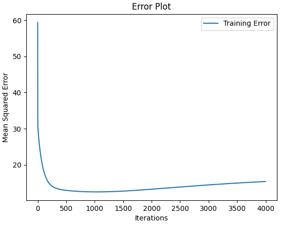
Mean squared error: 11.232800207362782 (given by reg. factor: 0.05)