Lasso回归于岭回归非常相似,它们的差别在于使用了不同的正则化项。最终都实现了约束参数从而防止过拟合的效果。但是Lasso之所以重要,还有另一个原因是:Lasso能够将一些作用比较小的特征的参数训练为0,从而获得稀疏解。也就是说用这种方法,在训练模型的过程中实现了降维(特征筛选)的目的。
Lasso回归的代价函数为:

上式中的w是长度为n的向量,不包括截距项的系数θ0, θ是长度为n+1的向量,包括截距项的系数θ0,m为样本数,n为特征数.||w||1表示参数w的l1范数,也是一种表示距离的函数。加入ww表示3维空间中的一个点(x,y,z),那么||w||1=|x|+|y|+|z|,即各个方向上的绝对值(长度)之和。
式子2−1的梯度为:
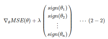
其中sign(θi)由θi的符号决定: θi>0,sign(θi)=1; θi=0,sign(θi)=0; θi<0,sign(θi)=−1θi>0,sign(θi)=1; θi=0,sign(θi)=0; θi<0,sign(θi)=−1.
上述解释摘自:https://www.cnblogs.com/Belter/p/8536939.html
接下来是实现代码,代码来源: https://github.com/eriklindernoren/ML-From-Scratch
首先还是定义一个基类,各种线性回归都需要继承该基类:
class Regression(object):
    """ Base regression model. Models the relationship between a scalar dependent variable y and the independent
    variables X.
    Parameters:
    -----------
    n_iterations: float
        The number of training iterations the algorithm will tune the weights for.
    learning_rate: float
        The step length that will be used when updating the weights.
    """
    def __init__(self, n_iterations, learning_rate):
        self.n_iterations = n_iterations
        self.learning_rate = learning_rate

    def initialize_weights(self, n_features):
        """ Initialize weights randomly [-1/N, 1/N] """
        limit = 1 / math.sqrt(n_features)
        self.w = np.random.uniform(-limit, limit, (n_features, ))

    def fit(self, X, y):
        # Insert constant ones for bias weights
        X = np.insert(X, 0, 1, axis=1)
        self.training_errors = []
        self.initialize_weights(n_features=X.shape[1])

        # Do gradient descent for n_iterations
        for i in range(self.n_iterations):
            y_pred = X.dot(self.w)
            # Calculate l2 loss
            mse = np.mean(0.5 * (y - y_pred)**2 + self.regularization(self.w))
            self.training_errors.append(mse)
            # Gradient of l2 loss w.r.t w
            grad_w = -(y - y_pred).dot(X) + self.regularization.grad(self.w)
            # Update the weights
            self.w -= self.learning_rate * grad_w

    def predict(self, X):
        # Insert constant ones for bias weights
        X = np.insert(X, 0, 1, axis=1)
        y_pred = X.dot(self.w)
        return y_pred
需要注意的是这里的mse损失函数前面就只是0.5。
lasso回归的核心就是l1正则化,其代码如下所示:
class l1_regularization():
    """ Regularization for Lasso Regression """
    def __init__(self, alpha):
        self.alpha = alpha

    def __call__(self, w):
        return self.alpha * np.linalg.norm(w)

    def grad(self, w):
        return self.alpha * np.sign(w)
然后是lasso回归代码:
class LassoRegression(Regression):
    """Linear regression model with a regularization factor which does both variable selection
    and regularization. Model that tries to balance the fit of the model with respect to the training
    data and the complexity of the model. A large regularization factor with decreases the variance of
    the model and do para.
    Parameters:
    -----------
    degree: int
        The degree of the polynomial that the independent variable X will be transformed to.
    reg_factor: float
        The factor that will determine the amount of regularization and feature
        shrinkage.
    n_iterations: float
        The number of training iterations the algorithm will tune the weights for.
    learning_rate: float
        The step length that will be used when updating the weights.
    """
    def __init__(self, degree, reg_factor, n_iterations=3000, learning_rate=0.01):
        self.degree = degree
        self.regularization = l1_regularization(alpha=reg_factor)
        super(LassoRegression, self).__init__(n_iterations,
                                            learning_rate)

    def fit(self, X, y):
        X = normalize(polynomial_features(X, degree=self.degree))
        super(LassoRegression, self).fit(X, y)

    def predict(self, X):
        X = normalize(polynomial_features(X, degree=self.degree))
        return super(LassoRegression, self).predict(X)
这里normalize()和polynomial_features()位于utils.data_manipulation下:
def normalize(X, axis=-1, order=2):
    """ Normalize the dataset X """
    l2 = np.atleast_1d(np.linalg.norm(X, order, axis))
    l2[l2 == 0] = 1
    return X / np.expand_dims(l2, axis)
np.linalg.norm():用于求范数,ord=order用于指定计算的范数类型。
np.atleast_1d():将输入的数据直接视为1维,比如输入的是1,那么经过该函数之后的输出就是[1]
def polynomial_features(X, degree):
    n_samples, n_features = np.shape(X)

    def index_combinations():
        combs = [combinations_with_replacement(range(n_features), i) for i in range(0, degree + 1)]
        flat_combs = [item for sublist in combs for item in sublist]
        return flat_combs

    combinations = index_combinations()
    n_output_features = len(combinations)
    X_new = np.empty((n_samples, n_output_features))

    for i, index_combs in enumerate(combinations):
        X_new[:, i] = np.prod(X[:, index_combs], axis=1)

    return X_new
这个是计算多项式特征函数。什么是多项式特征呢?
以sklearn中的为例:使用sklearn.preprocessing.PolynomialFeatures来进行特征的构造。它是使用多项式的方法来进行的,如果有a,b两个特征,那么它的2次多项式为(1,a,b,a^2,ab, b^2)。
PolynomialFeatures有三个参数
degree:控制多项式的度
interaction_only: 默认为False,如果指定为True,那么就不会有特征自己和自己结合的项,上面的二次项中没有a^2和b^2。
include_bias:默认为True。如果为True的话,那么就会有上面的 1那一项。
最后是使用:
首先是部分数据集:
time    temp
0.00273224    0.1
0.005464481    -4.5
0.008196721    -6.3
0.010928962    -9.6
0.013661202    -9.9
0.016393443    -17.1
0.019125683    -11.6
0.021857923    -6.2
0.024590164    -6.4
0.027322404    -0.5
0.030054645    0.5
0.032786885    -2.4
0.035519126    -7.5
然后是lasso回归的运行代码:
from __future__ import print_function
import sys
sys.path.append("/content/drive/My Drive/learn/ML-From-Scratch/")
import matplotlib.pyplot as plt
import numpy as np
import pandas as pd
# Import helper functions
from mlfromscratch.supervised_learning import LassoRegression
from mlfromscratch.utils import k_fold_cross_validation_sets, normalize, mean_squared_error
from mlfromscratch.utils import train_test_split, polynomial_features, Plot


def main():

    # Load temperature data
    data = pd.read_csv('mlfromscratch/data/TempLinkoping2016.txt', sep="	")

    time = np.atleast_2d(data["time"].values).T
    temp = data["temp"].values

    X = time # fraction of the year [0, 1]
    y = temp

    X_train, X_test, y_train, y_test = train_test_split(X, y, test_size=0.4)

    poly_degree = 13

    model = LassoRegression(degree=15,
                            reg_factor=0.05,
                            learning_rate=0.001,
                            n_iterations=4000)
    model.fit(X_train, y_train)

    # Training error plot
    n = len(model.training_errors)
    training, = plt.plot(range(n), model.training_errors, label="Training Error")
    plt.legend(handles=[training])
    plt.title("Error Plot")
    plt.ylabel('Mean Squared Error')
    plt.xlabel('Iterations')
    plt.show()

    y_pred = model.predict(X_test)
    mse = mean_squared_error(y_test, y_pred)
    print ("Mean squared error: %s (given by reg. factor: %s)" % (mse, 0.05))

    y_pred_line = model.predict(X)

    # Color map
    cmap = plt.get_cmap('viridis')

    # Plot the results
    m1 = plt.scatter(366 * X_train, y_train, color=cmap(0.9), s=10)
    m2 = plt.scatter(366 * X_test, y_test, color=cmap(0.5), s=10)
    plt.plot(366 * X, y_pred_line, color='black', linewidth=2, label="Prediction")
    plt.suptitle("Lasso Regression")
    plt.title("MSE: %.2f" % mse, fontsize=10)
    plt.xlabel('Day')
    plt.ylabel('Temperature in Celcius')
    plt.legend((m1, m2), ("Training data", "Test data"), loc='lower right')
    plt.show()

if __name__ == "__main__":
    main()
这里面也用到了utils下的很多函数,我们一一解析。
def train_test_split(X, y, test_size=0.5, shuffle=True, seed=None):
    """ Split the data into train and test sets """
    if shuffle:
        X, y = shuffle_data(X, y, seed)
    # Split the training data from test data in the ratio specified in
    # test_size
    split_i = len(y) - int(len(y) // (1 / test_size))
    X_train, X_test = X[:split_i], X[split_i:]
    y_train, y_test = y[:split_i], y[split_i:]

    return X_train, X_test, y_train, y_test
这里代码挺简单,里面还使用了:
def shuffle_data(X, y, seed=None):
    """ Random shuffle of the samples in X and y """
    if seed:
        np.random.seed(seed)
    idx = np.arange(X.shape[0])
    np.random.shuffle(idx)
    return X[idx], y[idx]
将数据进行打乱。
def k_fold_cross_validation_sets(X, y, k, shuffle=True):
    """ Split the data into k sets of training / test data """
    if shuffle:
        X, y = shuffle_data(X, y)

    n_samples = len(y)
    left_overs = {}
    n_left_overs = (n_samples % k)
    if n_left_overs != 0:
        left_overs["X"] = X[-n_left_overs:]
        left_overs["y"] = y[-n_left_overs:]
        X = X[:-n_left_overs]
        y = y[:-n_left_overs]

    X_split = np.split(X, k)
    y_split = np.split(y, k)
    sets = []
    for i in range(k):
        X_test, y_test = X_split[i], y_split[i]
        X_train = np.concatenate(X_split[:i] + X_split[i + 1:], axis=0)
        y_train = np.concatenate(y_split[:i] + y_split[i + 1:], axis=0)
        sets.append([X_train, X_test, y_train, y_test])

    # Add left over samples to last set as training samples
    if n_left_overs != 0:
        np.append(sets[-1][0], left_overs["X"], axis=0)
        np.append(sets[-1][2], left_overs["y"], axis=0)

    return np.array(sets)
进行k-fold交叉验证。
这里的这些函数在sklearn中都是有的,看这些代码可以加深理解。
结果:

Mean squared error: 11.302155412035969 (given by reg. factor: 0.05)
