Tensorflow-卷积神经网络CNN

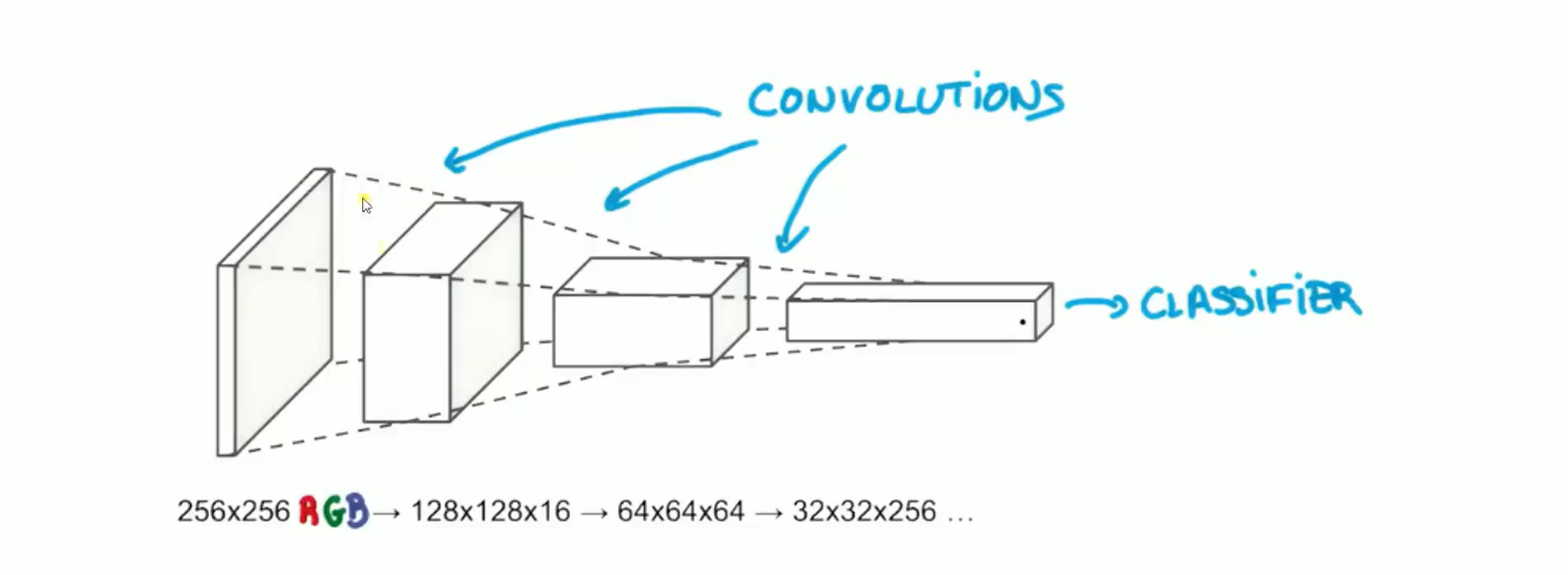
卷积神经网络CNN

结构

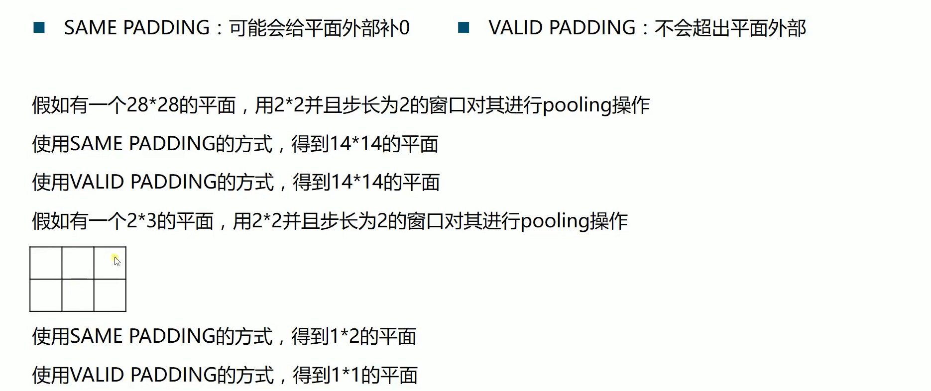
 池化操作

 手写数字-卷积神经网络实现

import tensorflow as tf
from tensorflow.examples.tutorials.mnist import input_data
tf.compat.v1.disable_eager_execution()
import numpy as np


#载入数据集
mnist=input_data.read_data_sets("MNIST_data",one_hot=True)

#每个批次大小
batch_size=100
#计算一共有多少个批次
n_bath=mnist.train.num_examples // batch_size

#初始化权值
def weight_variable(shape):
    initial=tf.compat.v1.truncated_normal(shape,stddev=0.1)#生成一个截断的正态分布
    return tf.Variable(initial)

#初始化偏置值
def bias_variable(shape):
    initial=tf.compat.v1.constant(0.1,shape=shape)#生成一个截断的正态分布
    return tf.Variable(initial)

#卷积层
def conv2d(x,W):
    #strides[0]=strides[3]=1,strides[1]代表x方向的步长，strides[2]代表y方向的步长
    return tf.nn.conv2d(x,W,strides=[1,1,1,1],padding='SAME')

#池化层
def max_pool_2x2(x):
    #ksize[1,x,y,1]
    return tf.nn.max_pool(x,ksize=[1,2,2,1],strides=[1,2,2,1],padding='SAME')

#定义两个placeholder
x=tf.compat.v1.placeholder(tf.float32,[None,784])#28*28
y=tf.compat.v1.placeholder(tf.float32,[None,10])

#改变x的格式转为4D的向量【batch,in_height,in_width,in_channels】
x_image=tf.compat.v1.reshape(x,[-1,28,28,1])

#初始化第一个卷积层的权值和偏置
W_conv1=weight_variable([5,5,1,32])#5*5的采样窗口，32个卷积核从1个平面抽取特征
b_conv1=bias_variable([32])#每一个卷积核一个偏置值

#把x_image和权值向量进行卷积，再加上偏置值，然后应用于relu激活函数
h_conv1=tf.nn.relu(conv2d(x_image,W_conv1)+b_conv1)
h_pool1=max_pool_2x2(h_conv1)#进行max-pooling

#初始化第二个卷积层的权值和偏置
W_conv2=weight_variable([5,5,32,64])#5*5的采样窗口，64个卷积核从32个平面抽取特征
b_conv2=bias_variable([64])#每一个卷积核一个偏置值

#把x_image和权值向量进行卷积，再加上偏置值，然后应用于relu激活函数
h_conv2=tf.nn.relu(conv2d(h_pool1,W_conv2)+b_conv2)
h_pool2=max_pool_2x2(h_conv2)#进行max-pooling

#28*28的图片第一次卷积后还是28*28（步长为1），第一次池化变为14*14（因为步长2）
#第二次卷积后为14*14，第二次池化为7*7
#经过以上步骤后得到64张7*7平面

#初始化第一个全连接层的权值
W_fc1=weight_variable([7*7*64,1024])#上一层有7*7*64个神经元，全连接层有1024个神经元
b_fc1=bias_variable([1024])#1024个节点

#把池化层的第二层输出扁平化为1维
h_pool2_flat=tf.compat.v1.reshape(h_pool2,[-1,7*7*64])
#求第一个全连接层的输出
h_fc1=tf.nn.relu(tf.matmul(h_pool2_flat,W_fc1)+b_fc1)

#用keep_prob来表示神经元的输出概率
# keep_prob=tf.compat.v1.placeholder(tf.float32)
# h_fc1_drop=tf.nn.dropout(h_fc1,keep_prob)


#初始化第二个全连接层的权值
W_fc2=weight_variable([1024,10])#上一层有7*7*64个神经元，全连接层有1024个神经元
b_fc2=bias_variable([10])#1024个节点

#计算输出
prediction=tf.nn.softmax(tf.matmul(h_fc1,W_fc2)+b_fc2)

#交叉熵函数
loss=tf.reduce_mean(tf.nn.softmax_cross_entropy_with_logits(labels=y,logits=prediction))
#梯度下降
train_step=tf.compat.v1.train.AdamOptimizer(1e-4).minimize(loss)

#初始化变量
init=tf.compat.v1.global_variables_initializer()

#结果存放在一个布尔型列表中
#返回的是一系列的True或False argmax返回一维张量中最大的值所在的位置，对比两个最大位置是否一致
correct_prediction=tf.equal(tf.argmax(y,1),tf.argmax(prediction,1))

#求准确率
#cast：将布尔类型转换为float，将True为1.0，False为0，然后求平均值
accuracy=tf.reduce_mean(tf.cast(correct_prediction,tf.float32))


with tf.compat.v1.Session() as sess:
    sess.run(init)
    for epoch in range(51):
        for batch in range(n_bath):
            #获得一批次的数据，batch_xs为图片，batch_ys为图片标签
            batch_xs,batch_ys=mnist.train.next_batch(batch_size)
            #进行训练
            sess.run(train_step,feed_dict={x:batch_xs,y:batch_ys})

        test_acc=sess.run(accuracy,feed_dict={x:mnist.test.images,y:mnist.test.labels})

        print("Iter "+str(epoch)+",Testing Accuracy "+str(test_acc))

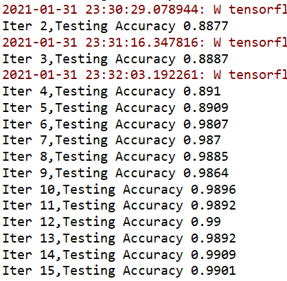
输出结果：

跑的时间有点长。。。。。