模型性能提升操作

 看了一些别人的思路，总结了一些模型性能提升的操作并完成python实现。

1. 行空缺值的处理

常规方法

统计每行数据的空缺值，如果空缺值数量超过阈值，则剔除此行数据。

改进方法

考虑特征重要度的因素。遵循一个原则：特征重要度越高，对这一特征下的空缺值容忍程度越低。

特征重要度的评估手段

1.1 输入特征方差膨胀系数或者方差

对特征归一化处理后，计算各特征方差膨胀系数或者方差。方差越大，说明这一特征数据波动性越大，对模型的贡献程度也就越高。试想一下，若一个特征的数据值全为1，则说明这一个特征对模型并没有产生什么贡献。

import pandas as pd
import numpy as np


def var_filter(data, label, k=0):
    """
    计算dataframe中输入特征方差并按阈值返回dataframe
    :param data: dataframe数据集，包括输入输出
    :param label: 输出特征
    :param k: 方差阈值
    :return:  按阈值返回dataframe
    """
    features = data.drop([label], axis=1).columns
    saved_features = []
    for feature in features:
        feature_var = np.array(data[feature]).var()
        print('输入特征{0}的方差为：{1}'.format(feature, feature_var))
        if feature_var > k:
            saved_features.append(feature)
    saved_features.append(label)
    filter_data = data[saved_features]
    return filter_data

1.2 输入特征共线性检验

所谓输入特征共线性即各特征之间存在线性相关的程度，共线性问题有如下几种检验方法：

相关性分析，检验变量之间的相关系数；

方差膨胀因子VIF，当VIF大于5或10时，代表模型存在严重的共线性问题；

条件数检验，当条件数大于100、1000时，代表模型存在严重的共线性问题。

这里，我们采用特征间皮尔逊相关系数作为共线性判断依据。

import pandas as pd
import numpy as np


def vif_test(data, label, k=None):
    """
    计算dataframe中输入特征之间的共线性系数
    :param data: dataframe数据集，包括输入输出
    :param label: 输出特征
    :param k: 相关系数阈值
    :return:  按阈值返回dataframe
    """
    features = data.drop([label], axis=1).columns
    feature_array = np.array(data[features])
    print(feature_array)
    vif_array = np.corrcoef(feature_array, rowvar=0)
    print(vif_array)
    for idx in range(len(features) - 1):
        for count in range(idx + 1, len(features)):
            vif = vif_array[idx][count]
            print('特征{0}与特征{1}的共线性系数vif为：{2}'.format(features[idx], features[count], vif))

1.3 输入特征与输出特征之间的皮尔逊相关系数

计算各输入特征与输出特征之间的皮尔逊相关系数，相关系数越高，说明特征的贡献程度越高，也就是说这一特征的重要度越大。

import pandas as pd
import numpy as np

def pearson_value(data, label, k=None):
    """
    计算dataframe中输入特征与输出特征之间的pearson相关系数并按阈值返回dataframe
    :param data: dataframe数据集，包括输入输出
    :param label: 输出特征
    :param k: 相关系数阈值
    :return:  按阈值返回dataframe
    """
    features = data.drop([label], axis=1).columns
    label_array = np.array(data[label])
    saved_features = []
    for feature in features:
        feature_array = np.array(data[feature])
        vstack = np.vstack([feature_array, label_array])
        pearson_coef = np.corrcoef(vstack)[0][1]
        print('输入特征{0}与输出特征{1}的皮尔逊相关系数为：{2}'.format(feature, label, pearson_coef))
        if pearson_coef > k:
            saved_features.append(feature)
    saved_features.append(label)
    filter_data = data[saved_features]
    return filter_data

1.4 互信息检验

计算各特征与输出特征之间的互信息( sklearn.metrics .mutual_info_score())

from sklearn import metrics as mr


def mutual_info(data, label, k=None):
    """
    计算dataframe中输入特征与输出特征之间的互信息mi并按阈值返回datframe
    :param data: dataframe数据集，包括输入输出
    :param label: 输出特征
    :param k: 相关系数阈值
    :return:  按阈值返回dataframe
    """
    features = data.drop([label], axis=1).columns
    label_array = np.array(data[label])
    saved_features = []
    for feature in features:
        feature_array = np.array(data[feature])
        mi = mr.mutual_info_score(label_array, feature_array)
        print('输入特征{0}与输出特征{1}的互信息为：{2}'.format(feature, label, mi))
        if mi > k:
            saved_features.append(feature)
    saved_features.append(label)
    filter_data = data[saved_features]
    return filter_data

1.5 在计算特征与输出特征之间的相关系数或者互信息的同时，考虑特征间的关系。

常用的方法如下：

1. Xgb’s importance
2. Logistic regression的params的参数
3. Recursive feature elimination（递归参数选择方法 RFE）
4. Pearson Correlation
5. Distance correlation

递归参数选择方法是通过考虑越来越小的特征集合来递归的选择特征。 首先，评估器在初始的特征集合上面训练并且每一个特征的重要程度是通过一个 coef_ 属性 或者 feature_importances_ 属性来获得。 然后，从当前的特征集合中移除最不重要的特征。在特征集合上不断的重复递归这个步骤，直到最终达到所需要的特征数量为止。

这里以xgb’s的 feature_importance_ 和 Recursive feature elimination（递归参数选择）为例，其中xgboost的python安装环境可以从 https://www.lfd.uci.edu/~gohlke/pythonlibs/#xgboost 选择对应的python版本下载。

xgboost提供了两种训练模型的API接口，分别是基于XGBoost的原生接口以及基于Scikit-learn接口。下面会各自用着两类接口分别做回归、分类模型的特征重要度展示及输出。

1.5.1 利用scikit-learn接口完成xgboost多分类模型训练及特征重要度展示：

import xgboost as xgb
from xgboost import plot_importance
from matplotlib import pyplot as plt
from sklearn.model_selection import train_test_split
from sklearn.metrics import accuracy_score


def xg_feature_importance(data, label):
    """
    利用scikit-learn接口完成xgboost多分类模型训练及特征重要度展示
    :param data: dataframe数据集，包括输入输出
    :param label: 输出特征
    :return:
    """
    X = np.array(data.drop([label], axis=1))
    y = np.array(data[label])
    X_train, X_test, y_train, y_test = train_test_split(X, y, test_size=0.2, random_state=0)
    # 训练分类模型
    model = xgb.XGBClassifier(max_depth=5, learning_rate=0.1, n_estimators=160, silent=True, objective='multi:softmax')
    model.fit(X_train, y_train)
    # 对测试集进行预测
    y_predict = model.predict(X_test)
    # 计算准确率
    accuracy = accuracy_score(y_test, y_predict)
    print("Accuracy: %.2f %% " % (100 * accuracy))
    # 显示重要特征
    plot_importance(model)
    plt.show()
    # 打印特征重要度
    print(model.feature_importances_)

1.5.2 利用scikit-learn接口完成xgboost回归模型训练及特征重要度展示：

import xgboost as xgb
from xgboost import plot_importance
from matplotlib import pyplot as plt
from sklearn.model_selection import train_test_split
from sklearn.metrics import mean_squared_error


def xg_feature_importance(data, label):
    """
    利用scikit-learn接口完成xgboost回归模型训练及特征重要度展示
    :param data: dataframe数据集，包括输入输出
    :param label: 输出特征
    :return:
    """
    X = np.array(data.drop([label], axis=1))
    y = np.array(data[label])
    # XGBoost训练过程
    X_train, X_test, y_train, y_test = train_test_split(X, y, test_size=0.2, random_state=0)
    params = {
        'booster': 'gbtree',
        'objective': 'reg:gamma',
        'gamma': 0.1,
        'max_depth': 5,
        'lambda': 3,
        'subsample': 0.7,
        'colsample_bytree': 0.7,
        'min_child_weight': 3,
        'silent': 1,
        'eta': 0.1,
        'seed': 1000,
        'nthread': 4,
    }

    dtrain = xgb.DMatrix(X_train, y_train)
    num_rounds = 126
    model = xgb.train(params, dtrain, num_rounds)
    # 对测试集进行预测
    dtest = xgb.DMatrix(X_test)
    y_predict = model.predict(dtest)
    # 计算MSE
    mse = mean_squared_error(y_test, y_predict)
    print("MSE: %.2f " % (mse))
    # 显示重要特征
    plot_importance(model)
    plt.show()
    # 打印特征重要度
    print(model.get_fscore().items())

1.5.3  利用scikit-learn 包里面的RFECV递归参数选择方法完成特征选择：

import matplotlib.pyplot as plt
from sklearn.svm import SVC
from sklearn.model_selection import StratifiedKFold
from sklearn.feature_selection import RFECV
from sklearn.datasets import make_classification


def rfecv(data, label):
    """
    递归参数选择方法 RFE计算特征重要度
    :param data:
    :param label:
    :return:
    """
    # Build a classification task using 3 informative features
    # X, y = make_classification(n_samples=1000, n_features=25, n_informative=3,
    #                            n_redundant=2, n_repeated=0, n_classes=8,
    #                            n_clusters_per_class=1, random_state=0)

    X = np.array(data.drop([label], axis=1))
    y = np.array(data[label])
    X_train, X_test, y_train, y_test = train_test_split(X, y, test_size=0.1, random_state=0)
    # Create the RFE object and compute a cross-validated score.
    svc = SVC(kernel="linear")
    # classifications
    rfecv = RFECV(estimator=svc, step=1, cv=StratifiedKFold(2),
                  scoring='accuracy')
    rfecv.fit(X_train, y_train)
    # 最佳特征数量
    print('最佳特征数量:{}'.format(rfecv.n_features_))
    # 每个特征的等级 ，估计最好的特征被分配到等级1。
    print('每个特征的排序等级:{}'.format(rfecv.ranking_))
    for idx, rank in enumerate(rfecv.ranking_):
        if rfecv.ranking_[idx] == 1:
            print('排序等级为1的特征是第{}个特征'.format(idx))
    # Plot number of features VS. cross-validation scores
    plt.figure()
    plt.xlabel("选择的特征数")
    plt.ylabel("交叉验证得分")
    plt.plot(range(1, len(rfecv.grid_scores_) + 1), rfecv.grid_scores_)
    plt.show()

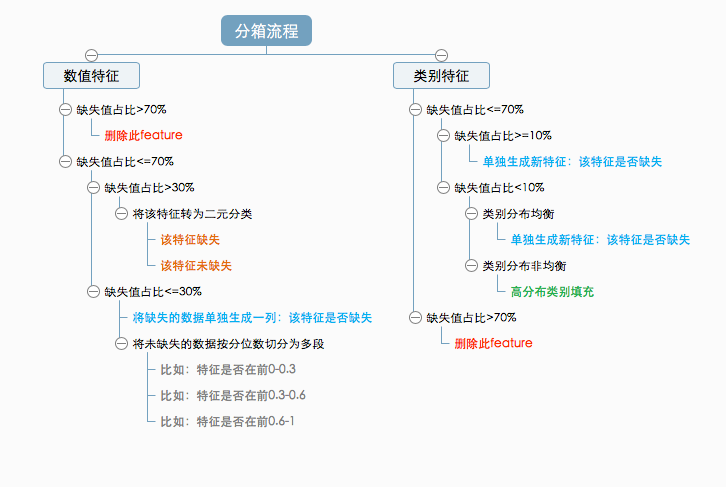
2. 列空缺值的处理

常规方法

观察特征数据分布，如果是连续变量且正态分布，用平均数或众数填充，如果偏态分布，用分位数填充。解释性相对不太强

改进方法

特征分箱。

特征分箱主要有以下优点 ： 

1. 可以将缺失作为独立的一类带入模型；
2. 稀疏向量内积乘法运算速度快，计算结果方便存储，容易扩展；
3. 保存了原始的信息，没有以填充或者删除的方式改变真实的数据分布；
4. 让特征存在的形式更加合理，比如age这个字段，其实我们在乎的不是27或者28这样的差别，而是90后，80后这样的差别，如果不采取分箱的形式，一定程度上夸大了27与26之前的差异；
5. 在数据计算中，不仅仅加快了计算的速度而且消除了实际数据记录中的随机偏差，平滑了存储过程中可能出现的噪音；

分箱操作示例（参考：数据分箱技术Binning）：

import numpy as np
import pandas as pd

# 对series分箱
score_list = np.random.randint(low=25, high=100, size=20)
# 分箱原则，规定：0-59为不及格，59-70为一般，70-80为良好，80-100位优秀：
bins = [0, 59, 70, 80, 100]
score_cut = pd.cut(score_list, bins)
# 统计各个段内数据的个数
pd.value_counts(score_cut)

# 对dataframe分箱
df = pd.DataFrame()
df['score'] = score_list
#    pd.util.testing.rands(3) for i in range(20)可以生成20个随机3位字符串。
df['student'] = [pd.util.testing.rands(3) for i in range(20)]
# 使用前面的bins标准对df进行分箱，得到一个categories 对象
df['categories'] = pd.cut(df['score'], bins, labels=['low', 'ok', 'good', 'great'])

3. 特征工程之特征交叉

在构造的具有可解释性特征的基础上，构造交叉特征，例如可以使用FM构造两两交叉特征（关于FM算法的部分，可以参考我的另一篇文章：FM算法解析及Python实现 ）。

需要注意的是，原始特征量较大的情况下，直接使用FM算法的方式进行特征构造，会使特征成倍增加。例如N个特征两两相乘，会产生N（N-1）/2个新特征。

所以，可以利用Xgboost或者随机森林对原始特征绘制特征重要度折线图，并重点关注拐点的特征，在拐点之间选择筛选出需要做交叉特征的原始特征及数量。从而减少交叉特征的大量出现。

4. 模型融合

模型融合不仅泛化性有提高，同时还会一定程度上提高预测的准确率，并且当模型融合中的基学习器之间互相独立时，模型融合的方法效果会更好。

常规方法

4.1 bagging

bagging 融合算法的目标是在每个子模块的设计选择过程中要尽可能的保证：

• low biase
• high var

也就是说子模块可以适当的过拟合，增加子模型拟合准确程度，通过加权平均的时候可以降低泛化误差

from sklearn.ensemble import BaggingClassifier
from sklearn.neighbors.classification import KNeighborsClassifier


def bag_class(x_train, y_train, max_samples, max_features, bootstrap, bootstrap_features, oob_score):
    """
    bagging method
    :param x_train: input trainset
    :param y_train: output trainset
    :param max_samples: The number of samples to draw from X to train each base estimator.
    :param max_features: The number of features to draw from X to train each base estimator.
    :param bootstrap: boolean, optional (default=True) Whether samples are drawn with replacement.
    :param bootstrap_features: boolean, optional (default=False) Whether features are drawn with replacement.
    :param oob_score: bool.Whether to use out-of-bag samples to estimate the generalization error.
    :return: bagging model
    """
    bagging = BaggingClassifier(KNeighborsClassifier(), max_samples=max_samples, max_features=max_features,
                                bootstrap=bootstrap, bootstrap_features=bootstrap_features, oob_score=oob_score)
    model = bagging.fit(x_train, y_train)
    return model

4.2 voting (bagging的改进型)

不同类型模型（树模型、线性模型、SVM等）通过硬投票或者软投票得到最终预测结果

from sklearn.ensemble import VotingClassifier
from sklearn.ensemble import GradientBoostingClassifier
from sklearn.naive_bayes import GaussianNB
from sklearn.ensemble import RandomForestClassifier


def voting_class(x_train, y_train, vote_type='hard', weights=None):
    """
    Voting Classifier
    voting by majority models or  voting by setting models weight of vote
    :param vote_type: 'hard' ,'soft'
    :param weights: list [1,2,1] or [2,1,2] etc  when set vote_type is 'soft'
    :return: classifier model
    """
    clf1 = GradientBoostingClassifier(random_state=1)
    clf2 = RandomForestClassifier(random_state=1)
    clf3 = GaussianNB()
    eclf = VotingClassifier(estimators=[('gbc', clf1), ('rf', clf2), ('gnb', clf3)], voting=vote_type,
                            weights=weights)
    model = eclf.fit(x_train, y_train)
    return model

4.3 boosting

改进方法

4.4 stacking方法

stacking融合算法的目标是在每个子模块1、子模块2的设计选择过程中要尽可能的保证：

• high biase
• low var

在子模块3的时候，要保证：

• low biase
• high var

也就是说，在子模块1，2的选择中，我们需要保证可稍欠拟合，在子模块3的拟合上再保证拟合的准确度及强度（增加树的深度max_depth、内部节点再划分所需最小样本数min_samples_split、叶子节点样本数min_samples_leaf、最大叶子节点数max_leaf_nodes等，可参考文章：scikit-learn 梯度提升树(GBDT)调参小结）

from sklearn import model_selection
from sklearn.neighbors import KNeighborsClassifier
from sklearn.ensemble import GradientBoostingClassifier
from sklearn.naive_bayes import GaussianNB
from sklearn.ensemble import RandomForestClassifier
from mlxtend.classifier import StackingClassifier


def stacking_class(x_train, y_train, use_probas=False, average_probas=False):
    """
    Stacking model ensemble
    basic model high biase and low var (underfitting),final model low biase and high var (overfitting)
    :param x_train: input trainset
    :param y_train: output trainset
    :param use_probas: True: the class probability generated from layer 1 basic classifier as the final total meta-classfier's input
                            False: the feature output generated by the basic classifier is used as the input of the final total meta-classifier
    :param average_probas: True: the probability value generated by the basic classifier for each category
                            will be averaged, otherwise(False) it will be spliced.
    :return: stacking model
    """

    clf1 = KNeighborsClassifier(n_neighbors=1)
    clf2 = RandomForestClassifier(random_state=1)
    clf3 = GaussianNB()
    # final model设计的overfitting 
    final_clf = GradientBoostingClassifier(max_depth=10,max_leaf_nodes=10)
    sclf = StackingClassifier(classifiers=[clf1, clf2, clf3],
                              use_probas=use_probas,
                              average_probas=average_probas,
                              meta_classifier=final_clf)
    for clf, label in zip([clf1, clf2, clf3, sclf],
                          ['KNN',
                           'Random Forest',
                           'Naive Bayes',
                           'StackingClassifier']):
        scores = model_selection.cross_val_score(clf, x_train, y_train,
                                                 cv=5, scoring='accuracy')
        print("Accuracy: %0.2f (+/- %0.2f) [%s]"
              % (scores.mean(), scores.std(), label))
    model = sclf.fit(x_train, y_train)
    return model

4.2 blending

我们知道单个组合子模块的结果不够理想，如果想得到更好的结果，需要把很多单个子模块的结果融合在一起：

这种方法也可以提高我们最后的预测的效果。