- "Natural parameter" links here. For the usage of this term in differential geometry, see differential geometry of curves.(微分几何曲线)
In probability and statistics, an exponential family is an important class of probability distributions sharing a certain form, specified below. This special form is chosen for mathematical convenience, on account of some useful algebraic properties, as well as for generality, as exponential families are in a sense very natural distributions to consider. The concept of exponential families is credited to[1] E. J. G. Pitman,[2] G. Darmois,[3] and B. O. Koopman[4] in 1935–6. The term exponential class is sometimes used in place of "exponential family".[5]
The exponential families include many of the most common distributions, including the normal, exponential, gamma, chi-squared, beta, Dirichlet,Bernoulli, binomial, multinomial, Poisson, and many others. Consideration of these, and other distributions that are with an exponential family of distributions, provides a framework for selecting a possible alternative parameterisation of the distribution, in terms of natural parameters, and for defining useful sample statistics, called the natural statistics of the family. See below for more information.
[edit]Definition
The following is a sequence of increasingly general definitions of an exponential family. A casual reader may wish to restrict attention to the first and simplest definition, which corresponds to a single-parameter family of discrete or continuous probability distributions.
[edit]Scalar parameter
A single-parameter exponential family is a set of probability distributions whose probability density function (or probability mass function, for the case of a discrete distribution) can be expressed in the form
![f_X(x|\theta) = h(x)\ \exp[\ \eta(\theta) \cdot T(x)\ -\ A(\theta)\ ]](http://upload.wikimedia.org/wikipedia/en/math/a/f/9/af9bd3c8e0bc577cd35494efeecb9013.png)
where T(x), h(x), η(θ), and A(θ) are known functions.
An alternative, equivalent form often given is
![f_X(x|\theta) = h(x)\ g(\theta) \exp[\ \eta(\theta) \cdot T(x)\ ]\,](http://upload.wikimedia.org/wikipedia/en/math/6/5/e/65e27dded8efde563d31c2197bd9fa73.png)
or equivalently
![f_X(x|\theta) = \exp[\ \eta(\theta) \cdot T(x)\ -\ A(\theta) + B(x)\ ]](http://upload.wikimedia.org/wikipedia/en/math/a/d/a/ada9bc54ad4787607ac7de22233192a4.png)
The value θ is called the parameter of the family.
Note that x is often a vector of measurements, in which case T(x) is a function from the space of possible values of x to the real numbers.
If η(θ) = θ, then the exponential family is said to be in canonical form. By defining a transformed parameter η = η(θ), it is always possible to convert an exponential family to canonical form. The canonical form is non-unique, since η(θ) can be multiplied by any nonzero constant, provided that T(x) is multiplied by that constant's reciprocal.
Even when x is a scalar, and there is only a single parameter, the functions η(θ) and T(x) can still be vectors, as described below.
Note also that the function A(θ) or equivalently g(θ) is automatically determined once the other functions have been chosen, and assumes a form that causes the distribution to be normalized (sum or integrate to one over the entire domain). Furthermore, both of these functions can always be written as functions of η, even when η(θ) is not a one-to-one function, i.e. two or more different values of θ map to the same value of η(θ), and hence η(θ) cannot be inverted. In such a case, all values of θ mapping to the same η(θ) will also have the same value for A(θ) and g(θ).
Further down the page is the example of a normal distribution with unknown mean and known variance.
[edit]Factorization of the variables involved
What is important to note, and what characterizes all exponential family variants, is that the parameter(s) and the observation variable(s) mustfactorize (can be separated into products each of which involves only one type of variable), either directly or within either part (the base or exponent) of an exponentiation operation. Generally, this means that all of the factors constituting the density or mass function must be of one of the following forms: f(x), g(θ), cf(x), cg(θ), [f(x)]c, [g(θ)]c, [f(x)]g(θ), [g(θ)]f(x), [f(x)]h(x)g(θ), or [g(θ)]h(x)j(θ), where f(x) and h(x) are arbitrary functions of x; g(θ) and j(θ)are arbitrary functions of θ; and c is an arbitrary "constant" expression (i.e. an expression not involving x or θ).
There are further restrictions on how many such factors can occur. For example, an expression of the sort [f(x)g(θ)]h(x)j(θ) is the same as[f(x)]h(x)j(θ)[g(θ)]h(x)j(θ), i.e. a product of two "allowed" factors. However, when rewritten into the factorized form,
![{[f(x) g(\theta)]}^{h(x)j(\theta)} = {[f(x)]}^{h(x)j(\theta)} [g(\theta)]^{h(x)j(\theta)} = e^{[h(x) \ln f(x)] j(\theta) + h(x) [j(\theta) \ln g(\theta)]}\, ,](http://upload.wikimedia.org/wikipedia/en/math/0/d/c/0dcf9f11a8e13799bdf0355f3d19a79f.png)
it can be seen that it cannot be expressed in the required form. (However, a form of this sort is a member of a curved exponential family, which allows multiple factorized terms in the exponent.[citation needed])
To see why an expression of the form [f(x)]g(θ) qualifies, note that
![{[f(x)]}^{g(\theta)} = e^{g(\theta) \ln f(x)}\,](http://upload.wikimedia.org/wikipedia/en/math/a/c/4/ac4e2c417c8602d3c7f4de77a2e17c53.png)
and hence factorizes inside of the exponent. Similarly,
![{[f(x)]}^{h(x)g(\theta)} = e^{h(x)g(\theta)\ln f(x)} = e^{[h(x) \ln f(x)] g(\theta)}\,](http://upload.wikimedia.org/wikipedia/en/math/7/2/d/72d3d06de7d5bda7b78d42f1fd782997.png)
and again factorizes inside of the exponent.
Note also that a factor consisting of a sum where both types of variables are involved (e.g. a factor of the form 1 + f(x)g(θ)) cannot be factorized in this fashion (except in some cases where occurring directly in an exponent); this is why, for example, the Cauchy distribution and Student's t distribution are not exponential families.
[edit]Vector parameter
The definition in terms of one real-number parameter can be extended to one real-vector parameter  . A family of distributions is said to belong to a vector exponential family if the probability density function (or probability mass function, for discrete distributions) can be written as
Or in a more compact form,
This form writes the sum as a dot product of vector-valued functions  and
and  .
.
An alternative, equivalent form often seen is
As in the scalar valued case, the exponential family is said to be in canonical form if  , for all i.
A vector exponential family is said to be curved if the dimension of is less than the dimension of the vector  . That is, if the dimension of the parameter vector is less than the number of functions of the parameter vector in the above representation of the probability density function. Note that most common distributions in the exponential family are not curved, and many algorithms designed to work with any member of the exponential family implicitly or explicitly assume that the distribution is not curved.
Note that, as in the above case of a scalar-valued parameter, the function  or equivalently
  is automatically determined once the other functions have been chosen, so that the entire distribution is normalized. In addition, as above, both of these functions can always be written as functions of
  , regardless of the form of the transformation that generates from
  . Hence an exponential family in its "natural form" (parametrized by its natural parameter) looks like

or equivalently

Note that the above forms may sometimes be seen with  in place of
  . These are exactly equivalent formulations, merely using different notation for the dot product.
Further down the page is the example of a normal distribution with unknown mean and variance.
[edit]Vector parameter, vector variable
The vector-parameter form over a single scalar-valued random variable can be trivially expanded to cover a joint distribution over a vector of random variables. The resulting distribution is simply the same as the above distribution for a scalar-valued random variable with each occurrence of the scalarx replaced by the vector  . Note that the dimension k of the random variable need not match the dimension d of the parameter vector, nor (in the case of a curved exponential function) the dimension s of the natural parameter and sufficient statistic
  .
.
The distribution in this case is written as

Or more compactly as

Or alternatively as

[edit]Measure-theoretic formulation
We use cumulative distribution functions (cdf) in order to encompass both discrete and continuous distributions.
Suppose H is a non-decreasing function of a real variable. Then Lebesgue–Stieltjes integrals with respect to dH(x) are integrals with respect to the "reference measure" of the exponential family generated by H.
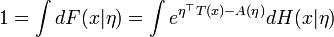
Any member of that exponential family has cumulative distribution function

If F is a continuous distribution with a density, one can write dF(x) = f(x) dx.
H(x) is a Lebesgue–Stieltjes integrator for the reference measure. When the reference measure is finite, it can be normalized and H is actually thecumulative distribution function of a probability distribution. If F is absolutely continuous with a density, then so is H, which can then be writtendH(x) = h(x) dx. If F is discrete, then H is a step function (with steps on the support of F).
[edit]Interpretation
In the definitions above, the functions T(x), η(θ), and A(η) were apparently arbitrarily defined. However, these functions play a significant role in the resulting probability distribution.
- T(x) is a sufficient statistic of the distribution. Thus, for exponential families, there exists a sufficient statistic whose dimension equals the number of parameters to be estimated. This important property is further discussed below.
- η is called the natural parameter. The set of values of η for which the function fX(x;θ) is finite is called the natural parameter space. It can be shown that the natural parameter space is always convex.
- A(η) is a normalization factor, or log-partition function, without which fX(x;θ) would not be a probability distribution. The function A is important in its own right, because K(u|η) = A(η + u) − A(η) is the cumulant generating function of the sufficient statistic T(x). This means one can fully understand the mean and covariance structure of T = (T1, T2, ... , Tp) by differentiating A(η).
[edit]Examples
The normal, exponential, gamma, chi-squared, beta, Weibull, Dirichlet, Bernoulli, binomial, multinomial, Poisson, negative binomial (with known parameterr), and geometric distributions are all exponential families. The family of Pareto distributions with a fixed minimum bound form an exponential family.
The Cauchy and uniform families of distributions are not exponential families. The Laplace family is not an exponential family unless the mean is zero.
Following are some detailed examples of the representation of some useful distribution as exponential families.
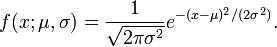
[edit]Normal distribution: Unknown mean, known variance
As a first example, consider a random variable distributed normally with unknown mean μ and known variance σ2. The probability density function is then
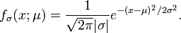
This is a single-parameter exponential family, as can be seen by setting
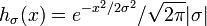

If σ = 1 this is in canonical form, as then η(μ) = μ.
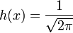
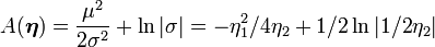
[edit]Normal distribution: Unknown mean and unknown variance
Next, consider the case of a normal distribution with unknown mean and unknown variance. The probability density function is then
This is an exponential family which can be written in canonical form by defining


[edit]Binomial distribution
As an example of a discrete exponential family, consider the binomial distribution with known number of trials n. The probability mass function for this distribution is
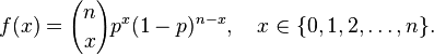
This can equivalently be written as
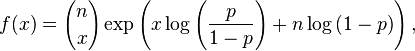
which shows that the binomial distribution is an exponential family, whose natural parameter is

This function of p is known as logit.
[edit]Moments and cumulants of the sufficient statistic
[edit]Normalization of the distribution
We start with the normalization of the probability distribution. Since
it follows that

This justifies calling A the log-partition function.
[edit]Moment generating function of the sufficient statistic
Now, the moment generating function of T(x) is
![M_T(u) \equiv E[e^{u^\top T(x)}|\eta] = \int e^{(\eta+u)^\top T(x)-A(\eta)}dH(x|\eta) = e^{A(\eta + u)-A(\eta)}](http://upload.wikimedia.org/wikipedia/en/math/a/0/0/a00a81537d99a93de6900a4aac1799af.png)
proving the earlier statement that K(u | η) = A(η + u) − A(η) is the cumulant generating function for T.
An important subclass of the exponential family the natural exponential family has a similar form for the moment generating function for the distribution of x.
[edit]Differential identities for cumulants
In particular,

and
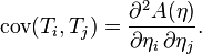
The first two raw moments and all mixed second moments can be recovered from these two identities. Higher order moments and cumulants are obtained by higher derivatives. This technique is often useful when T is a complicated function of the data, whose moments are difficult to calculate by integration.
[edit]Example
As an example consider a real valued random variable  with density

indexed by shape parameter  (this is called the skew-logistic distribution). The density can be rewritten as

Notice this is an exponential family with natural parameter

sufficient statistic
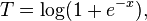
and normalizing factor

So using the first identity,
![E(\log(1 + e^{-X})) = E(T) = \frac{ \partial A(\eta) }{ \partial \eta } = \frac{ \partial }{ \partial \eta } [-\log(-\eta)] = \frac{1}{-\eta} = \frac{1}{\theta},](http://upload.wikimedia.org/wikipedia/en/math/2/7/8/27832487e4e82360bbe55c71ddbe01da.png)
and using the second identity
![\mathrm{var}(\log(1 + e^{-X})) = \frac{ \partial^2 A(\eta) }{ \partial \eta^2 } = \frac{ \partial }{ \partial \eta } \left[\frac{1}{-\eta}\right] = \frac{1}{(-\eta)^2} = \frac{1}{\theta^2}.](http://upload.wikimedia.org/wikipedia/en/math/0/5/b/05b270bca9b3bf6456a33359b09518b0.png)
This example illustrates a case where using this method is very simple, but the direct calculation would be nearly impossible.
[edit]Maximum entropy derivation
The exponential family arises naturally as the answer to the following question: what is the maximum-entropy distribution consistent with given constraints on expected values?
The information entropy of a probability distribution dF(x) can only be computed with respect to some other probability distribution (or, more generally, a positive measure), and both measures must be mutually absolutely continuous. Accordingly, we need to pick a reference measure dH(x) with the same support as dF(x). As an aside, frequentists need to realize that this is a largely arbitrary choice, while Bayesians can just make this choice part of their prior probability distribution.
The entropy of dF(x) relative to dH(x) is
![S[dF|dH]=-\int {dF\over dH}\ln{dF\over dH}\,dH](http://upload.wikimedia.org/wikipedia/en/math/5/e/f/5efc2cdb67b140dbc87572875a028bb2.png)
or
![S[dF|dH]=\int\ln{dH\over dF}\,dF](http://upload.wikimedia.org/wikipedia/en/math/2/9/6/29631dbc474d8acf46fc11d365054146.png)
where dF/dH and dH/dF are Radon–Nikodym derivatives. Note that the ordinary definition of entropy for a discrete distribution supported on a set I, namely
assumes, though this is seldom pointed out, that dH is chosen to be the counting measure on I.
Consider now a collection of observable quantities (random variables) Ti. The probability distribution dF whose entropy with respect to dH is greatest, subject to the conditions that the expected value of Ti be equal to ti, is a member of the exponential family with dH as reference measure and (T1, ...,Tn) as sufficient statistic.
The derivation is a simple variational calculation using Lagrange multipliers. Normalization is imposed by letting T0 = 1 be one of the constraints. The natural parameters of the distribution are the Lagrange multipliers, and the normalization factor is the Lagrange multiplier associated to T0.
For examples of such derivations, see Maximum entropy probability distribution.
[edit]Role in statistics
[edit]Classical estimation: sufficiency
According to the Pitman–Koopman–Darmois theorem, among families of probability distributions whose domain does not vary with the parameter being estimated, only in exponential families is there a sufficient statistic whose dimension remains bounded as sample size increases. Less tersely, supposeXn, n = 1, 2, 3, ... are independent identically distributed random variables whose distribution is known to be in some family of probability distributions. Only if that family is an exponential family is there a (possibly vector-valued) sufficient statistic T(X1, ..., Xn) whose number of scalar components does not increase as the sample size n increases.
[edit]Bayesian estimation: conjugate distributions
Exponential families are also important in Bayesian statistics. In Bayesian statistics a prior distribution is multiplied by a likelihood function and then normalised to produce a posterior distribution. In the case of a likelihood which belongs to the exponential family there exists a conjugate prior, which is often also in the exponential family. A conjugate prior π for the parameter of an exponential family is given by

or equivalently

where  (where s is the dimension of ) and ν > 0 are hyperparameters (parameters controlling parameters). ν corresponds to the effective number of observations that the prior distribution contributes, and
  corresponds to the total amount that these pseudo-observations contribute to thesufficient statistic over all observations and pseudo-observations.
  is a normalization constant that is automatically determined by the remaining functions and serves to ensure that the given function is a probability density function (i.e. it is normalized).
  and equivalently
  are the same functions as in the definition of the distribution over which π is the conjugate prior.
A conjugate prior is one which, when combined with the likelihood and normalised, produces a posterior distribution which is of the same type as the prior. For example, if one is estimating the success probability of a binomial distribution, then if one chooses to use a beta distribution as one's prior, the posterior is another beta distribution. This makes the computation of the posterior particularly simple. Similarly, if one is estimating the parameter of a Poisson distribution the use of a gamma prior will lead to another gamma posterior. Conjugate priors are often very flexible and can be very convenient. However, if one's belief about the likely value of the theta parameter of a binomial is represented by (say) a bimodal (two-humped) prior distribution, then this cannot be represented by a beta distribution. It can however be represented by using a mixture density as the prior, here a combination of two beta distributions; this is a form of hyperprior.
An arbitrary likelihood will not belong to the exponential family, and thus in general no conjugate prior exists. The posterior will then have to be computed by numerical methods.
[edit]Hypothesis testing: Uniformly most powerful tests
The one-parameter exponential family has a monotone non-decreasing likelihood ratio in the sufficient statistic T(x), provided that η(θ) is non-decreasing. As a consequence, there exists a uniformly most powerful test for testing the hypothesis H0: θ ≥ θ0 vs. H1: θ < θ0.
[edit]Generalized linear models
The exponential family forms the basis for the distribution function used in generalized linear models, a class of model that encompass many of the commonly used regression models in statistics.