在本教程中,把注意力转向 TVM 如何使用张量表达式(Tensor Expression,简称 TE)定义张量计算并应用循环优化。TE 以纯函数式语言描述张量计算(即每个表达式都没有副作用)。从 TVM 的整体来看,Relay 将计算描述为一组算子,这些算子都可以表示为 TE 表达式,每个 TE 表达式都接受输入张量并生成输出张量。
TVM使用一个特定领域的张量表达式来进行有效的内核构建。我们将通过两个使用张量表达语言的例子来演示基本的工作流程。第一个例子介绍了TE和向量加法进行调度。第二部分对这些概念进行了扩展,逐步优化了一个带TE的矩阵乘法。这个矩阵乘法的例子将作为未来涵盖TVM更高级功能的教程的比较基础。
Example 1: Writing and Scheduling Vector Addition in TE for CPU
将实现一个向量加法的TE,然后是一个针对CPU的时间表。
首先初始化一个TVM环境
import tvm
import tvm.testing
from tvm import te
import numpy as np
如果能够明确指明目标的CPU并指明它,将会得到更好的性能。如果你使用 LLVM,你可以从命令llc --version中得到这个信息,以获得 CPU 类型,你可以检查 /proc/cpuinfo,了解你的处理器可能支持的额外扩展。。例如,你可以使用 llvm -mcpu=skylake-avx512 来获取带有 AVX-512 指令的 CPU。
tgt = tvm.target.Target(target="llvm", host="llvm")
Describing the Vector Computation
此处描述了一个向量加法的计算。TVM采用张量语义,每个中间结果都表示一个多维数组。用户需要描述生成张量的计算规则。首先定义一个符号变量n来表示形状。然后定义两个占位张量,A和B,具有给定的形状(n,)。然后我们描述结果张量C,并进行compute操作。compute定义了一个计算,输出符合指定的张量形状,计算将在张量中由lambda函数定义的每个位置进行。
Note: 虽然n是一个变量,但它定义了A、B和C张量之间的一致形状。
Remember: 这个阶段并没有实际的计算产生,因为只是声明了如何进行计算
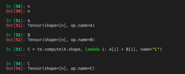
n = te.var("n")
A = te.placeholder((n,), name="A")
B = te.placeholder((n,), name="B")
C = te.compute(A.shape, lambda i: A[i] + B[i], name="C")
Lambda函数
te.compute方法的第二个参数是执行计算的函数。在这个例子中,使用一个匿名函数,也被称为 lambda 函数,来定义计算,在本例中是对A和B的第i个元素进行加法。
Create a Default Schedule for the Computation
虽然上面几行描述了计算规则,但我们可以使用不同的方式计算C,以适应不同的设备。对于有多个轴的张量,你可以选择先迭代哪个轴,或者将计算分给不同的线程。TVM要求使用者提供一个schedule,它描述了如何进行计算。TE中的Schedule操作可以改变循环顺序,在不同的线程中分割计算,并将数据块分组以及其他 操作。Schedule背后的一个重要概念就是,它们只描述了计算是如何进行的,所以同一个TE的不同Schedule会产生相同的结果。
TVM允许创建一个本地的schedule,通过以行为主的顺序迭代计算C
for (int i = 0; i < n; ++i) {
  C[i] = A[i] + B[i];
}
s = te.create_schedule(C.op)
Compile and Evaluate the Default Schedule
有了TE表达式和schedule,便可为我们目标语言和架构(这里是LLVM和CPU)生产可运行的代码。向TVM提供Schedule/Schedule中的TE表达式列表/目标和主机以及要生成的函数名称。输出的结果是一个类型消除的函数,可以直接从Python中调用。
在下面的一行,使用tvm.build来创建一个函数。构建的函数需要schedule/所需的函数签名(包括输入和输出)以及想要编译的目标语言。
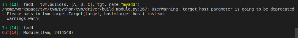
fadd = tvm.build(s, [A, B, C], tgt, name="myadd")
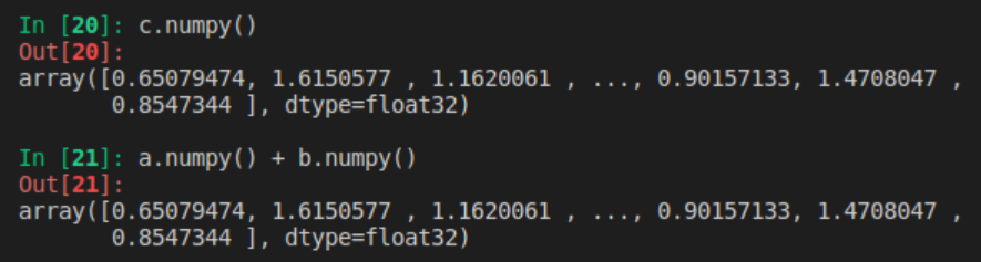
运行下面的函数,并将其输出与numpy中的相同计算进行比较。编译后的TVM函数暴露了一个简洁的C语言API,可以从任何语言调用。首先创建一个设备(本例中为CPU),TVM能够将Schedule编译到设备上。在本例中,该设备就是LLVM CPU目标,然后初始化设备中的张量,并执行自定义加法运算。为验证计算是否正确,可以将C张量的输出结果与numpy进行的相同计算进行比较。
dev = tvm.device(tgt.kind.name, 0)

n = 1024
a = tvm.nd.array(np.random.uniform(size=n).astype(A.dtype), dev)
b = tvm.nd.array(np.random.uniform(size=n).astype(B.dtype), dev)
c = tvm.nd.array(np.zeros(n, dtype=C.dtype), dev)
fadd(a, b, c)
tvm.testing.assert_allclose(c.numpy(), a.numpy() + b.numpy())
运行结果:
为了比较这个版本与numpy哪个更快,创建了一个辅助函数来运行TVM生成代码的配置文件
import timeit

np_repeat = 100
np_running_time = timeit.timeit(
    setup="import numpy\n"
    "n = 32768\n"
    'dtype = "float32"\n'
    "a = numpy.random.rand(n, 1).astype(dtype)\n"
    "b = numpy.random.rand(n, 1).astype(dtype)\n",
    stmt="answer = a + b",
    number=np_repeat,
)
print("Numpy running time: %f" % (np_running_time / np_repeat))


def evaluate_addition(func, target, optimization, log):
    dev = tvm.device(target.kind.name, 0)
    n = 32768
    a = tvm.nd.array(np.random.uniform(size=n).astype(A.dtype), dev)
    b = tvm.nd.array(np.random.uniform(size=n).astype(B.dtype), dev)
    c = tvm.nd.array(np.zeros(n, dtype=C.dtype), dev)

    evaluator = func.time_evaluator(func.entry_name, dev, number=10)
    mean_time = evaluator(a, b, c).mean
    print("%s: %f" % (optimization, mean_time))

    log.append((optimization, mean_time))


log = [("numpy", np_running_time / np_repeat)]
evaluate_addition(fadd, tgt, "naive", log=log)
输出结果:
Numpy running time: 0.000004
naive: 0.000005
PS:
不知道为什么,本地跑的结果竟然numpy比生成的这个版本运行时间还短,惊呆了,重复多次,还是这个结果,虽有浮动,但最好的也是和Numpy运行时间一样,也许笔记本的性能太好了吧,哈哈哈
Updating the Schedule to Use Parallelism
现在已经基本说明了TE的基本原理,本小节将更深入地了解schedule的作用,以及如何使用它来优化不同架构的张量表达。Schedule是应用于表达式的一系列步骤,以多种不同方式对其进行转换。当Schedule被应用于TE的表达式时,输入/输出保持不变,但当编译时,表达式的实现将发生变化。默认的Schedule中,向量加法是串行运行,但很容易在所有的处理器线程中进行并行化。可以在我们的计算中应用并行Schedule 操作。
看到现在,似乎并没有说明schedule到底是个什么东西?
TVM借鉴了Halide中计算逻辑和调度分离的思想。Schedule可看作一系列优化措施的集合,它不会改变计算结果,但通过选取合适的策略来提高计算的性能。
TVM中关于调度原语(Schedule Primitives)的文档见这里。我们可以参考Halide中关于Schedule的描述,它提供了可视化的动图,便于更直观的了解。
参考:图解TVM中的调度原语(Schedule Primitives)
s[C].parallel(C.op.axis[0])
tvm.lower命令将生成TE的中间表示(IR),以及对应的schedule.通过应用不同的调度操作来lower expression,可以看到调度对计算排序的影响。使用标志simple_mode=True返回一个可读的C风格语句
print(tvm.lower(s, [A, B, C], simple_mode=True))
结果如下:
@main = primfn(A_1: handle, B_1: handle, C_1: handle) -> ()
  attr = {"from_legacy_te_schedule": True, "global_symbol": "main", "tir.noalias": True}
  buffers = {A: Buffer(A_2: Pointer(float32), float32, [(stride: int32*n: int32)], [], type="auto"),
             B: Buffer(B_2: Pointer(float32), float32, [(stride_1: int32*n)], [], type="auto"),
             C: Buffer(C_2: Pointer(float32), float32, [(stride_2: int32*n)], [], type="auto")}
  buffer_map = {A_1: A, B_1: B, C_1: C}
  preflattened_buffer_map = {A_1: A_3: Buffer(A_2, float32, [n], [stride], type="auto"), B_1: B_3: Buffer(B_2, float32, [n], [stride_1], type="auto"), C_1: C_3: Buffer(C_2, float32, [n], [stride_2], type="auto")} {
  for (i: int32, 0, n) "parallel" {
    C[(i*stride_2)] = (A[(i*stride)] + B[(i*stride_1)])
  }
}
现在,TVM有可能在独立的线程上运行这些块。让我们编译并运行这个应用了并行操作的新调度。
fadd_parallel = tvm.build(s, [A, B, C], tgt, name="myadd_parallel")
fadd_parallel(a, b, c)

tvm.testing.assert_allclose(c.numpy(), a.numpy() + b.numpy())

evaluate_addition(fadd_parallel, tgt, "parallel", log=log)
运行解果:
/home/workspace/tvm/tvm/python/tvm/driver/build_module.py:267: UserWarning: target_host parameter is going to be deprecated. Please pass in tvm.target.Target(target, host=target_host) instead.
  warnings.warn(
parallel: 0.000002
Updating the Schedule to Use Vectorization
现代CPU有能力对浮点值进行SIMD运算(Single Instruction Multiple Data,SIMD 即单指令多数据流 ),可以对我们的计算表达式应用另一个调度,以利用这个优势。完成这一点需要多个步骤:首先,必须使用分割调度原语(he split scheduling primitive)将调度分割成内循环和外循环。 内循环可以使用矢量化调度原语来使用SIMD指令,然后外循环可以使用并行调度原语进行并行化。选择分割因子为你的 CPU 上的线程数。
# Recreate the schedule, since we modified it with the parallel operation in
# the previous example
n = te.var("n")
A = te.placeholder((n,), name="A")
B = te.placeholder((n,), name="B")
C = te.compute(A.shape, lambda i: A[i] + B[i], name="C")

s = te.create_schedule(C.op)

# This factor should be chosen to match the number of threads appropriate for
# your CPU. This will vary depending on architecture, but a good rule is
# setting this factor to equal the number of available CPU cores.
factor = 4

outer, inner = s[C].split(C.op.axis[0], factor=factor)
s[C].parallel(outer)
s[C].vectorize(inner)

fadd_vector = tvm.build(s, [A, B, C], tgt, name="myadd_parallel")

evaluate_addition(fadd_vector, tgt, "vector", log=log)

print(tvm.lower(s, [A, B, C], simple_mode=True))
运行结果:
/home/workspace/tvm/tvm/python/tvm/driver/build_module.py:267: UserWarning: target_host parameter is going to be deprecated. Please pass in tvm.target.Target(target, host=target_host) instead.
  warnings.warn(
vector: 0.000015
@main = primfn(A_1: handle, B_1: handle, C_1: handle) -> ()
  attr = {"from_legacy_te_schedule": True, "global_symbol": "main", "tir.noalias": True}
  buffers = {A: Buffer(A_2: Pointer(float32), float32, [(stride: int32*n: int32)], [], type="auto"),
             B: Buffer(B_2: Pointer(float32), float32, [(stride_1: int32*n)], [], type="auto"),
             C: Buffer(C_2: Pointer(float32), float32, [(stride_2: int32*n)], [], type="auto")}
  buffer_map = {A_1: A, B_1: B, C_1: C}
  preflattened_buffer_map = {A_1: A_3: Buffer(A_2, float32, [n], [stride], type="auto"), B_1: B_3: Buffer(B_2, float32, [n], [stride_1], type="auto"), C_1: C_3: Buffer(C_2, float32, [n], [stride_2], type="auto")} {
  for (i.outer: int32, 0, floordiv((n + 3), 4)) "parallel" {
    for (i.inner.s: int32, 0, 4) {
      if @tir.likely((((i.outer*4) + i.inner.s) < n), dtype=bool) {
        let cse_var_1: int32 = ((i.outer*4) + i.inner.s)
        C[(cse_var_1*stride_2)] = (A[(cse_var_1*stride)] + B[(cse_var_1*stride_1)])
      }
    }
  }
}
Comparing the Different Schedules
现在比较不同的调度
baseline = log[0][1]
print("%s\t%s\t%s" % ("Operator".rjust(20), "Timing".rjust(20), "Performance".rjust(20)))
for result in log:
    print(
        "%s\t%s\t%s"
        % (result[0].rjust(20), str(result[1]).rjust(20), str(result[1] / baseline).rjust(20))
    )
输出结果:
          Operator                  Timing             Performance
               numpy    3.948449157178402e-06                    1.0
               naive              3.9715e-06      1.0058379484967386
            parallel                4.32e-06      1.0941004500833214
              vector              7.6747e-06      1.9437251676514966
可看到vector的性能提高了不少。
PS:
可以在计算声明中写 n = tvm.runtime.convert(1024),而不是 n = te.var("n") 。生成的函数将只接受长度为 1024 的向量。
上面我们已经定义/调度(schedule)/编译了一个向量加法算子,然后我们能够在TVM runtime运行它。可以将算子保存为一个库,可以在以后TVM runtime 加载使用它。
Targeting Vector Addition for GPUs (Optional)
TVM是能够针对多架构的。下个例子中,将针对GPU的向量加法进行编译。
# If you want to run this code, change ``run_cuda = True``
# Note that by default this example is not run in the docs CI.

run_cuda = False
if run_cuda:
    # Change this target to the correct backend for you gpu. For example: cuda (NVIDIA GPUs),
    # rocm (Radeon GPUS), OpenCL (opencl).
    tgt_gpu = tvm.target.Target(target="cuda", host="llvm")

    # Recreate the schedule
    n = te.var("n")
    A = te.placeholder((n,), name="A")
    B = te.placeholder((n,), name="B")
    C = te.compute(A.shape, lambda i: A[i] + B[i], name="C")
    print(type(C))

    s = te.create_schedule(C.op)

    bx, tx = s[C].split(C.op.axis[0], factor=64)

    ################################################################################
    # Finally we must bind the iteration axis bx and tx to threads in the GPU
    # compute grid. The naive schedule is not valid for GPUs, and these are
    # specific constructs that allow us to generate code that runs on a GPU.

    s[C].bind(bx, te.thread_axis("blockIdx.x"))
    s[C].bind(tx, te.thread_axis("threadIdx.x"))

    ######################################################################
    # Compilation
    # -----------
    # After we have finished specifying the schedule, we can compile it
    # into a TVM function. By default TVM compiles into a type-erased
    # function that can be directly called from the python side.
    #
    # In the following line, we use tvm.build to create a function.
    # The build function takes the schedule, the desired signature of the
    # function (including the inputs and outputs) as well as target language
    # we want to compile to.
    #
    # The result of compilation fadd is a GPU device function (if GPU is
    # involved) as well as a host wrapper that calls into the GPU
    # function. fadd is the generated host wrapper function, it contains
    # a reference to the generated device function internally.

    fadd = tvm.build(s, [A, B, C], target=tgt_gpu, name="myadd")

    ################################################################################
    # The compiled TVM function exposes a concise C API that can be invoked from
    # any language.
    #
    # We provide a minimal array API in python to aid quick testing and prototyping.
    # The array API is based on the `DLPack <https://github.com/dmlc/dlpack>`_ standard.
    #
    # - We first create a GPU device.
    # - Then tvm.nd.array copies the data to the GPU.
    # - ``fadd`` runs the actual computation
    # - ``numpy()`` copies the GPU array back to the CPU (so we can verify correctness).
    #
    # Note that copying the data to and from the memory on the GPU is a required step.

    dev = tvm.device(tgt_gpu.kind.name, 0)

    n = 1024
    a = tvm.nd.array(np.random.uniform(size=n).astype(A.dtype), dev)
    b = tvm.nd.array(np.random.uniform(size=n).astype(B.dtype), dev)
    c = tvm.nd.array(np.zeros(n, dtype=C.dtype), dev)
    fadd(a, b, c)
    tvm.testing.assert_allclose(c.numpy(), a.numpy() + b.numpy())

    ################################################################################
    # Inspect the Generated GPU Code
    # ~~~~~~~~~~~~~~~~~~~~~~~~~~~~~~
    # You can inspect the generated code in TVM. The result of tvm.build is a TVM
    # Module. fadd is the host module that contains the host wrapper, it also
    # contains a device module for the CUDA (GPU) function.
    #
    # The following code fetches the device module and prints the content code.

    if (
        tgt_gpu.kind.name == "cuda"
        or tgt_gpu.kind.name == "rocm"
        or tgt_gpu.kind.name.startswith("opencl")
    ):
        dev_module = fadd.imported_modules[0]
        print("-----GPU code-----")
        print(dev_module.get_source())
    else:
        print(fadd.get_source())
运行结果:

Saving and Loading Compiled Modules
除了运行时编译,我们还可以将编译后的模块保存到一个文件中,以后再加载回来。
执行步骤如下:
- 编译后的host module 保存到一个对象文件中。
- 然后它将设备模块保存到 ptx 文件中。
cc.create_shared调用编译器(gcc)来创建共享库
from tvm.contrib import cc
from tvm.contrib import utils

temp = utils.tempdir()
fadd.save(temp.relpath("myadd.o"))
if tgt.kind.name == "cuda":
    fadd.imported_modules[0].save(temp.relpath("myadd.ptx"))
if tgt.kind.name == "rocm":
    fadd.imported_modules[0].save(temp.relpath("myadd.hsaco"))
if tgt.kind.name.startswith("opencl"):
    fadd.imported_modules[0].save(temp.relpath("myadd.cl"))
cc.create_shared(temp.relpath("myadd.so"), [temp.relpath("myadd.o")])
print(temp.listdir())
运行结果:
['myadd.o', 'myadd.so']
CPU(主机)模块被直接保存为共享库(.so)。设备代码可以有多种自定义格式。在我们的例子中,设备代码被保存在 ptx 中,还有一个元数据 json 文件。它们可以通过导入分离加载和链接。
temp.relpath()接口:
Load Compiled Module
我们可以从文件系统中加载编译好的模块并运行代码。下面的代码分别加载主机和设备模块,并将它们链接在一起。我们可以验证新加载的功能是否工作。
fadd1 = tvm.runtime.load_module(temp.relpath("myadd.so"))
if tgt.kind.name == "cuda":
    fadd1_dev = tvm.runtime.load_module(temp.relpath("myadd.ptx"))
    fadd1.import_module(fadd1_dev)

if tgt.kind.name == "rocm":
    fadd1_dev = tvm.runtime.load_module(temp.relpath("myadd.hsaco"))
    fadd1.import_module(fadd1_dev)

if tgt.kind.name.startswith("opencl"):
    fadd1_dev = tvm.runtime.load_module(temp.relpath("myadd.cl"))
    fadd1.import_module(fadd1_dev)

fadd1(a, b, c)
tvm.testing.assert_allclose(c.numpy(), a.numpy() + b.numpy())
Pack Everything into One Library
上面的例子,分别存储了设备和主机代码,TVM也支持将所有东西打包成一个*.so文件。在底层,将设备模块打包成二进制代码,并将他们与主机代码链接起来。目前,支持Meta/OpenCL和Cuda模块的打包
fadd.export_library(temp.relpath("myadd_pack.so"))
fadd2 = tvm.runtime.load_module(temp.relpath("myadd_pack.so"))
fadd2(a, b, c)
tvm.testing.assert_allclose(c.numpy(), a.numpy() + b.numpy())
PS:运行时 API 和线程安全
TVM 的编译模块并不依赖于 TVM 编译器。相反,它们只依赖于一个最小的运行时库。TVM 运行库包装了设备驱动程序,并提供线程安全和设备无关的调用到编译的函数。
这意味着你可以从任何线程、任何 GPU 上调用已编译的 TVM 函数,只要你已经为该 GPU 编译了代码。
Generate OpenCL Code
TVM 提供代码生成功能到多个后端。我们还可以生成 OpenCL 代码或 LLVM 代码,在 CPU 后端运行。
下面的代码块生成 OpenCL 代码,在 OpenCL 设备上创建阵列,并验证代码的正确性。
if tgt.kind.name.startswith("opencl"):
    fadd_cl = tvm.build(s, [A, B, C], tgt, name="myadd")
    print("------opencl code------")
    print(fadd_cl.imported_modules[0].get_source())
    dev = tvm.cl(0)
    n = 1024
    a = tvm.nd.array(np.random.uniform(size=n).astype(A.dtype), dev)
    b = tvm.nd.array(np.random.uniform(size=n).astype(B.dtype), dev)
    c = tvm.nd.array(np.zeros(n, dtype=C.dtype), dev)
    fadd_cl(a, b, c)
    tvm.testing.assert_allclose(c.numpy(), a.numpy() + b.numpy())
PS:
TE调度原语
TVM 包括一些不同的调度原语:
split:将一个指定的轴按定义的因子(factor)分成两个轴。

tile:将一个计算按定义的 factor 分成两个轴。

fuse:融合一个计算的两个连续轴。

reorder:可以将一个计算的轴重新排序到一个定义的顺序。

bind:可以将一个计算绑定到一个特定的线程,在GPU编程中很有用。

compute_at:默认情况下,TVM 会在函数的最外层计算张量,也就是默认的根。compute_at 指定一个张量应该在另一个运算符的第一个计算轴上计算。

compute_inline:当标记为内联时,一个计算将被展开,然后插入到需要张量的地址中。

compute_root:将一个计算移到函数的最外层,或根部。这意味着该阶段的计算将在进入下一阶段之前被完全计算。
这些原语的完整描述可以在 Schedule Primitives文档页中找到。
Example 2: Manually Optimizing Matrix Multiplication with TE
考虑一个更高级的例子,演示仅用18行python代码,TVM如何将一个普通的矩阵乘法操作加快 18 倍。
矩阵乘法是一个计算密集型操作。为了获得良好的 CPU 性能,有两个重要的优化措施:
-
提高内存访问的高速缓存命中率。
复杂的数值计算和热点内存(hot-spot memory)访问都可以通过高缓存命中率(high cache hit rate)来加速。这就要求将原内存访问模式转化为符合缓存策略的模式。 -
SMID(Single instruction multi-data),也被成为向量处理单元。
在每个周期,SIMD可以处理一小批数据,而不是处理单个数值。这需要将循环体中的数据访问模式转化为统一模式,以便LLVM后端能够降低到SIMD
本教程中使用的技术是本资源库中提到的技巧的一个子集。其中一些已经被TVM抽象自动应用了,但由于TVM的限制,其中一些不能自动应用。
Preparation and Performance Baseline
首先收集numpy实现矩阵乘法的性能数据。
import tvm
import tvm.testing
from tvm import te
import numpy

# The size of the matrix
# (M, K) x (K, N)
# You are free to try out different shapes, sometimes TVM optimization outperforms numpy with MKL.
M = 1024
K = 1024
N = 1024

# The default tensor data type in tvm
dtype = "float32"

# You will want to adjust the target to match any CPU vector extensions you
# might have. For example, if you're using using Intel AVX2 (Advanced Vector
# Extensions) ISA for SIMD, you can get the best performance by changing the
# following line to ``llvm -mcpu=core-avx2``, or specific type of CPU you use.
# Recall that you're using llvm, you can get this information from the command
# ``llc --version`` to get the CPU type, and you can check ``/proc/cpuinfo``
# for additional extensions that your processor might support.

target = tvm.target.Target(target="llvm", host="llvm")
dev = tvm.device(target.kind.name, 0)

# Random generated tensor for testing
a = tvm.nd.array(numpy.random.rand(M, K).astype(dtype), dev)
b = tvm.nd.array(numpy.random.rand(K, N).astype(dtype), dev)

# Repeatedly perform a matrix multiplication to get a performance baseline
# for the default numpy implementation
np_repeat = 100
np_running_time = timeit.timeit(
    setup="import numpy\n"
    "M = " + str(M) + "\n"
    "K = " + str(K) + "\n"
    "N = " + str(N) + "\n"
    'dtype = "float32"\n'
    "a = numpy.random.rand(M, K).astype(dtype)\n"
    "b = numpy.random.rand(K, N).astype(dtype)\n",
    stmt="answer = numpy.dot(a, b)",
    number=np_repeat,
)
print("Numpy running time: %f" % (np_running_time / np_repeat))

answer = numpy.dot(a.numpy(), b.numpy())
运行结果:
Numpy running time: 0.003806
answer输出结果:
array([[264.74338, 262.21436, 255.64435, ..., 255.5698 , 254.58826,
        260.0738 ],
       [256.29956, 255.10828, 250.9674 , ..., 246.4632 , 247.5887 ,
        252.08322],
       [263.81436, 267.0429 , 259.11823, ..., 263.9015 , 267.28546,
        262.65903],
       ...,
       [251.28212, 255.52078, 251.23851, ..., 253.57953, 254.76633,
        254.243  ],
       [261.22546, 251.66624, 245.57074, ..., 245.58075, 252.56612,
        249.00397],
       [264.2958 , 262.14423, 255.72536, ..., 265.50284, 257.86594,
        257.44412]], dtype=float32)
现在使用TVM TE写一个基本的矩阵乘法,并验证它的结果与numpy是否相同。同样写了一个函数,帮助衡量调度优化的性能。
# TVM Matrix Multiplication using TE
k = te.reduce_axis((0, K), "k")
A = te.placeholder((M, K), name="A")
B = te.placeholder((K, N), name="B")
C = te.compute((M, N), lambda x, y: te.sum(A[x, k] * B[k, y], axis=k), name="C")

# Default schedule
s = te.create_schedule(C.op)
func = tvm.build(s, [A, B, C], target=target, name="mmult")

c = tvm.nd.array(numpy.zeros((M, N), dtype=dtype), dev)
func(a, b, c)
tvm.testing.assert_allclose(c.numpy(), answer, rtol=1e-5)


def evaluate_operation(s, vars, target, name, optimization, log):
    func = tvm.build(s, [A, B, C], target=target, name="mmult")
    assert func

    c = tvm.nd.array(numpy.zeros((M, N), dtype=dtype), dev)
    func(a, b, c)
    tvm.testing.assert_allclose(c.numpy(), answer, rtol=1e-5)

    evaluator = func.time_evaluator(func.entry_name, dev, number=10)
    mean_time = evaluator(a, b, c).mean
    print("%s: %f" % (optimization, mean_time))
    log.append((optimization, mean_time))


log = []

evaluate_operation(s, [A, B, C], target=target, name="mmult", optimization="none", log=log)
运行结果:
/home/workspace/tvm/tvm/python/tvm/driver/build_module.py:267: UserWarning: target_host parameter is going to be deprecated. Please pass in tvm.target.Target(target, host=target_host) instead.
  warnings.warn(
none: 1.934404
使用TVM lower函数来看下算子和默认调度的中间表达。注意:这个实现基本上是矩阵乘法的笨的实现,在A和B矩阵的索引上使用三个嵌套循环。
print(tvm.lower(s, [A, B, C], simple_mode=True))
输出结果:
@main = primfn(A_1: handle, B_1: handle, C_1: handle) -> ()
  attr = {"from_legacy_te_schedule": True, "global_symbol": "main", "tir.noalias": True}
  buffers = {A: Buffer(A_2: Pointer(float32), float32, [1048576], []),
             B: Buffer(B_2: Pointer(float32), float32, [1048576], []),
             C: Buffer(C_2: Pointer(float32), float32, [1048576], [])}
  buffer_map = {A_1: A, B_1: B, C_1: C}
  preflattened_buffer_map = {A_1: A_3: Buffer(A_2, float32, [1024, 1024], []), B_1: B_3: Buffer(B_2, float32, [1024, 1024], []), C_1: C_3: Buffer(C_2, float32, [1024, 1024], [])} {
  for (x: int32, 0, 1024) {
    for (y: int32, 0, 1024) {
      C[((x*1024) + y)] = 0f32
      for (k: int32, 0, 1024) {
        let cse_var_2: int32 = (x*1024)
        let cse_var_1: int32 = (cse_var_2 + y)
        C[cse_var_1] = (C[cse_var_1] + (A[(cse_var_2 + k)]*B[((k*1024) + y)]))
      }
    }
  }
}
Optimization 1: Blocking
提高缓冲区命中率的一个重要技巧是阻塞,在这个过程中,你的内存访问结构是在一个块的内部有一个小的邻域,具有很高的内存定位性。选择一个 32 的块因子。这将导致一个块充满 32 * 32 * sizeof(float) 的内存区域。这相当于一个 4KB的缓存大小,而 L1 缓存的参考缓存大小为 32KB。
首先为C操作创建一个默认的调度,然后用指定的block factor ,调用一个title调度基元。调度基元返回所产生的循环顺序,从最外层到最内层,作为一个向量[x_outer, y_outer, x_inner, y_inner]。然后为操作的输出获取到reduction axis,并使用 4 的因子对其进行分割操作。这个因子并不直接影响正在进行的阻塞优化操作,但在应用矢量化时会很有用。
现在操作已经被阻塞了,可以重新调度计算的顺序,把reduction operation放到计算的最外层中,保证被阻塞的数据仍在缓存中,这样就完成了调度,可以建立并测试与原生的调度相比的性能。
bn = 32

# Blocking by loop tiling
xo, yo, xi, yi = s[C].tile(C.op.axis[0], C.op.axis[1], bn, bn)
(k,) = s[C].op.reduce_axis
ko, ki = s[C].split(k, factor=4)

# Hoist reduction domain outside the blocking loop
s[C].reorder(xo, yo, ko, ki, xi, yi)

evaluate_operation(s, [A, B, C], target=target, name="mmult", optimization="blocking", log=log)
运行结果:
/home/workspace/tvm/tvm/python/tvm/driver/build_module.py:267: UserWarning: target_host parameter is going to be deprecated. Please pass in tvm.target.Target(target, host=target_host) instead.
  warnings.warn(
blocking: 0.128212
通过重新安排计算顺序充分利用缓存,可看到计算性能有了明显的改善。通过lower函数查看中间表达并与原始的进行比较:
print(tvm.lower(s, [A, B, C], simple_mode=True))
输出结果:
@main = primfn(A_1: handle, B_1: handle, C_1: handle) -> ()
  attr = {"from_legacy_te_schedule": True, "global_symbol": "main", "tir.noalias": True}
  buffers = {A: Buffer(A_2: Pointer(float32), float32, [1048576], []),
             B: Buffer(B_2: Pointer(float32), float32, [1048576], []),
             C: Buffer(C_2: Pointer(float32), float32, [1048576], [])}
  buffer_map = {A_1: A, B_1: B, C_1: C}
  preflattened_buffer_map = {A_1: A_3: Buffer(A_2, float32, [1024, 1024], []), B_1: B_3: Buffer(B_2, float32, [1024, 1024], []), C_1: C_3: Buffer(C_2, float32, [1024, 1024], [])} {
  for (x.outer: int32, 0, 32) {
    for (y.outer: int32, 0, 32) {
      for (x.inner.init: int32, 0, 32) {
        for (y.inner.init: int32, 0, 32) {
          C[((((x.outer*32768) + (x.inner.init*1024)) + (y.outer*32)) + y.inner.init)] = 0f32
        }
      }
      for (k.outer: int32, 0, 256) {
        for (k.inner: int32, 0, 4) {
          for (x.inner: int32, 0, 32) {
            for (y.inner: int32, 0, 32) {
              let cse_var_3: int32 = (y.outer*32)
              let cse_var_2: int32 = ((x.outer*32768) + (x.inner*1024))
              let cse_var_1: int32 = ((cse_var_2 + cse_var_3) + y.inner)
              C[cse_var_1] = (C[cse_var_1] + (A[((cse_var_2 + (k.outer*4)) + k.inner)]*B[((((k.outer*4096) + (k.inner*1024)) + cse_var_3) + y.inner)]))
            }
          }
        }
      }
    }
  }
}
Optimization 2: Vectorization
另一个重要的优化技巧是vectorization矢量化。当内存访问模式是统一的,编译器可以检测到这种模式并将连续的内存传递给SIMD矢量处理器。在TVM中,可以使用vectorize接口来提示编译器使用这种模式,充分利用硬件特性
我们选择对内循环的行数据进行矢量处理,因为在我们之前的优化中,它已经对缓存友好了。
# Apply the vectorization optimization
s[C].vectorize(yi)

evaluate_operation(s, [A, B, C], target=target, name="mmult", optimization="vectorization", log=log)

# The generalized IR after vectorization
print(tvm.lower(s, [A, B, C], simple_mode=True))
运行结果:
vectorization: 0.134151

@main = primfn(A_1: handle, B_1: handle, C_1: handle) -> ()
  attr = {"from_legacy_te_schedule": True, "global_symbol": "main", "tir.noalias": True}
  buffers = {A: Buffer(A_2: Pointer(float32), float32, [1048576], []),
             B: Buffer(B_2: Pointer(float32), float32, [1048576], []),
             C: Buffer(C_2: Pointer(float32), float32, [1048576], [])}
  buffer_map = {A_1: A, B_1: B, C_1: C}
  preflattened_buffer_map = {A_1: A_3: Buffer(A_2, float32, [1024, 1024], []), B_1: B_3: Buffer(B_2, float32, [1024, 1024], []), C_1: C_3: Buffer(C_2, float32, [1024, 1024], [])} {
  for (x.outer: int32, 0, 32) {
    for (y.outer: int32, 0, 32) {
      for (x.inner.init: int32, 0, 32) {
        C[ramp((((x.outer*32768) + (x.inner.init*1024)) + (y.outer*32)), 1, 32)] = broadcast(0f32, 32)
      }
      for (k.outer: int32, 0, 256) {
        for (k.inner: int32, 0, 4) {
          for (x.inner: int32, 0, 32) {
            let cse_var_3: int32 = (y.outer*32)
            let cse_var_2: int32 = ((x.outer*32768) + (x.inner*1024))
            let cse_var_1: int32 = (cse_var_2 + cse_var_3)
            C[ramp(cse_var_1, 1, 32)] = (C[ramp(cse_var_1, 1, 32)] + (broadcast(A[((cse_var_2 + (k.outer*4)) + k.inner)], 32)*B[ramp((((k.outer*4096) + (k.inner*1024)) + cse_var_3), 1, 32)]))
          }
        }
      }
    }
  }
}
Optimization 3: Loop Permutation
如果看了上面的IR,可以看到内循环的行数据被矢量化,B被转化为PackedB(这从内循环的(float32x32*)B2部分可以看出)。现在 PackedB 的遍历是顺序的。所以要看一下 A 的访问模式。在当前的计划中,A 是被逐列访问的,这对缓冲区不友好。如果改变 ki 和内轴 xi 的嵌套循环顺序,A 矩阵的访问模式将对缓存更友好。
s = te.create_schedule(C.op)
xo, yo, xi, yi = s[C].tile(C.op.axis[0], C.op.axis[1], bn, bn)
(k,) = s[C].op.reduce_axis
ko, ki = s[C].split(k, factor=4)

# re-ordering
s[C].reorder(xo, yo, ko, xi, ki, yi)
s[C].vectorize(yi)

evaluate_operation(
    s, [A, B, C], target=target, name="mmult", optimization="loop permutation", log=log
)

# Again, print the new generalized IR
print(tvm.lower(s, [A, B, C], simple_mode=True))
运行结果:
loop permutation: 0.074337

@main = primfn(A_1: handle, B_1: handle, C_1: handle) -> ()
  attr = {"from_legacy_te_schedule": True, "global_symbol": "main", "tir.noalias": True}
  buffers = {A: Buffer(A_2: Pointer(float32), float32, [1048576], []),
             B: Buffer(B_2: Pointer(float32), float32, [1048576], []),
             C: Buffer(C_2: Pointer(float32), float32, [1048576], [])}
  buffer_map = {A_1: A, B_1: B, C_1: C}
  preflattened_buffer_map = {A_1: A_3: Buffer(A_2, float32, [1024, 1024], []), B_1: B_3: Buffer(B_2, float32, [1024, 1024], []), C_1: C_3: Buffer(C_2, float32, [1024, 1024], [])} {
  for (x.outer: int32, 0, 32) {
    for (y.outer: int32, 0, 32) {
      for (x.inner.init: int32, 0, 32) {
        C[ramp((((x.outer*32768) + (x.inner.init*1024)) + (y.outer*32)), 1, 32)] = broadcast(0f32, 32)
      }
      for (k.outer: int32, 0, 256) {
        for (x.inner: int32, 0, 32) {
          for (k.inner: int32, 0, 4) {
            let cse_var_3: int32 = (y.outer*32)
            let cse_var_2: int32 = ((x.outer*32768) + (x.inner*1024))
            let cse_var_1: int32 = (cse_var_2 + cse_var_3)
            C[ramp(cse_var_1, 1, 32)] = (C[ramp(cse_var_1, 1, 32)] + (broadcast(A[((cse_var_2 + (k.outer*4)) + k.inner)], 32)*B[ramp((((k.outer*4096) + (k.inner*1024)) + cse_var_3), 1, 32)]))
          }
        }
      }
    }
  }
}
Optimization 4: Array Packing
另一个重要的技巧是数组打包。这个技巧是对数组的存储维度进行重新排序,将某些维度上的连续访问模式转换为扁平化后的顺序模式。
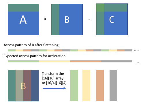
正如上图所示,在阻塞计算后,我们可以观察到 B 的数组访问模式(扁平化后),它是有规律的,但是不连续的。我们期望经过一些转换后,我们可以得到一个连续的访问模式。通过将[16][16]数组重新排序为[16/4][16][4]数组,当从打包的数组中抓取相应的值时,B 的访问模式将是连续的。
为了实现这一目标,将不得不从新的默认调度开始,考虑到 B 的新包装,值得花点时间来评论一下。TE 是编写优化运算符的强大而富有表现力的语言,但它往往需要对你所编写的底层算法、数据结构和硬件目标有一些了解。在本教程的后面,我们将讨论一些让 TVM 承担这一负担的选项。无论如何,让我们继续编写新的优化调度。
# We have to re-write the algorithm slightly.
packedB = te.compute((N / bn, K, bn), lambda x, y, z: B[y, x * bn + z], name="packedB")
C = te.compute(
    (M, N),
    lambda x, y: te.sum(A[x, k] * packedB[y // bn, k, tvm.tir.indexmod(y, bn)], axis=k),
    name="C",
)

s = te.create_schedule(C.op)

xo, yo, xi, yi = s[C].tile(C.op.axis[0], C.op.axis[1], bn, bn)
(k,) = s[C].op.reduce_axis
ko, ki = s[C].split(k, factor=4)

s[C].reorder(xo, yo, ko, xi, ki, yi)
s[C].vectorize(yi)

x, y, z = s[packedB].op.axis
s[packedB].vectorize(z)
s[packedB].parallel(x)

evaluate_operation(s, [A, B, C], target=target, name="mmult", optimization="array packing", log=log)

# Here is the generated IR after array packing.
print(tvm.lower(s, [A, B, C], simple_mode=True))
输出结果:
array packing: 0.082546

@main = primfn(A_1: handle, B_1: handle, C_1: handle) -> ()
  attr = {"from_legacy_te_schedule": True, "global_symbol": "main", "tir.noalias": True}
  buffers = {A: Buffer(A_2: Pointer(float32), float32, [1048576], []),
             B: Buffer(B_2: Pointer(float32), float32, [1048576], []),
             C: Buffer(C_2: Pointer(float32), float32, [1048576], [])}
  buffer_map = {A_1: A, B_1: B, C_1: C}
  preflattened_buffer_map = {A_1: A_3: Buffer(A_2, float32, [1024, 1024], []), B_1: B_3: Buffer(B_2, float32, [1024, 1024], []), C_1: C_3: Buffer(C_2, float32, [1024, 1024], [])} {
  allocate(packedB: Pointer(global float32x32), float32x32, [32768]), storage_scope = global {
    for (x: int32, 0, 32) "parallel" {
      for (y: int32, 0, 1024) {
        packedB_1: Buffer(packedB, float32x32, [32768], [])[((x*1024) + y)] = B[ramp(((y*1024) + (x*32)), 1, 32)]
      }
    }
    for (x.outer: int32, 0, 32) {
      for (y.outer: int32, 0, 32) {
        for (x.inner.init: int32, 0, 32) {
          C[ramp((((x.outer*32768) + (x.inner.init*1024)) + (y.outer*32)), 1, 32)] = broadcast(0f32, 32)
        }
        for (k.outer: int32, 0, 256) {
          for (x.inner: int32, 0, 32) {
            for (k.inner: int32, 0, 4) {
              let cse_var_3: int32 = ((x.outer*32768) + (x.inner*1024))
              let cse_var_2: int32 = (k.outer*4)
              let cse_var_1: int32 = (cse_var_3 + (y.outer*32))
              C[ramp(cse_var_1, 1, 32)] = (C[ramp(cse_var_1, 1, 32)] + (broadcast(A[((cse_var_3 + cse_var_2) + k.inner)], 32)*packedB_1[(((y.outer*1024) + cse_var_2) + k.inner)]))
            }
          }
        }
      }
    }
  }
}
Optimization 5: Optimizing Block Writing Through Caching
到目前为止,我们所有的优化都集中在有效地访问和计算 A 和 B 矩阵的数据以计算C矩阵上。在阻塞优化之后,运算器将逐块地将结果写入 C,而且访问模式不是顺序的。我们可以通过使用一个顺序缓存数组来解决这个问题,使用 cache_write、compute_at 和 unroll 的组合来保存块结果,并在所有块结果准备好后写入 C。
s = te.create_schedule(C.op)

# Allocate write cache
CC = s.cache_write(C, "global")

xo, yo, xi, yi = s[C].tile(C.op.axis[0], C.op.axis[1], bn, bn)

# Write cache is computed at yo
s[CC].compute_at(s[C], yo)

# New inner axes
xc, yc = s[CC].op.axis

(k,) = s[CC].op.reduce_axis
ko, ki = s[CC].split(k, factor=4)
s[CC].reorder(ko, xc, ki, yc)
s[CC].unroll(ki)
s[CC].vectorize(yc)

x, y, z = s[packedB].op.axis
s[packedB].vectorize(z)
s[packedB].parallel(x)

evaluate_operation(s, [A, B, C], target=target, name="mmult", optimization="block caching", log=log)

# Here is the generated IR after write cache blocking.
print(tvm.lower(s, [A, B, C], simple_mode=True))
输出结果:
block caching: 0.065276
@main = primfn(A_1: handle, B_1: handle, C_1: handle) -> ()
  attr = {"from_legacy_te_schedule": True, "global_symbol": "main", "tir.noalias": True}
  buffers = {A: Buffer(A_2: Pointer(float32), float32, [1048576], []),
             B: Buffer(B_2: Pointer(float32), float32, [1048576], []),
             C: Buffer(C_2: Pointer(float32), float32, [1048576], [])}
  buffer_map = {A_1: A, B_1: B, C_1: C}
  preflattened_buffer_map = {A_1: A_3: Buffer(A_2, float32, [1024, 1024], []), B_1: B_3: Buffer(B_2, float32, [1024, 1024], []), C_1: C_3: Buffer(C_2, float32, [1024, 1024], [])} {
  allocate(packedB: Pointer(global float32x32), float32x32, [32768]), storage_scope = global;
  allocate(C.global: Pointer(global float32), float32, [1024]), storage_scope = global {
    for (x: int32, 0, 32) "parallel" {
      for (y: int32, 0, 1024) {
        packedB_1: Buffer(packedB, float32x32, [32768], [])[((x*1024) + y)] = B[ramp(((y*1024) + (x*32)), 1, 32)]
      }
    }
    for (x.outer: int32, 0, 32) {
      for (y.outer: int32, 0, 32) {
        for (x.c.init: int32, 0, 32) {
          C.global_1: Buffer(C.global, float32, [1024], [])[ramp((x.c.init*32), 1, 32)] = broadcast(0f32, 32)
        }
        for (k.outer: int32, 0, 256) {
          for (x.c: int32, 0, 32) {
            let cse_var_4: int32 = (k.outer*4)
            let cse_var_3: int32 = (x.c*32)
            let cse_var_2: int32 = ((y.outer*1024) + cse_var_4)
            let cse_var_1: int32 = (((x.outer*32768) + (x.c*1024)) + cse_var_4)
             {
              C.global_1[ramp(cse_var_3, 1, 32)] = (C.global_1[ramp(cse_var_3, 1, 32)] + (broadcast(A[cse_var_1], 32)*packedB_1[cse_var_2]))
              C.global_1[ramp(cse_var_3, 1, 32)] = (C.global_1[ramp(cse_var_3, 1, 32)] + (broadcast(A[(cse_var_1 + 1)], 32)*packedB_1[(cse_var_2 + 1)]))
              C.global_1[ramp(cse_var_3, 1, 32)] = (C.global_1[ramp(cse_var_3, 1, 32)] + (broadcast(A[(cse_var_1 + 2)], 32)*packedB_1[(cse_var_2 + 2)]))
              C.global_1[ramp(cse_var_3, 1, 32)] = (C.global_1[ramp(cse_var_3, 1, 32)] + (broadcast(A[(cse_var_1 + 3)], 32)*packedB_1[(cse_var_2 + 3)]))
            }
          }
        }
        for (x.inner: int32, 0, 32) {
          for (y.inner: int32, 0, 32) {
            C[((((x.outer*32768) + (x.inner*1024)) + (y.outer*32)) + y.inner)] = C.global_1[((x.inner*32) + y.inner)]
          }
        }
      }
    }
  }
}
Optimization 6: Parallelization
到目前为止,我们的计算只被设计为使用单核。几乎所有的现代处理器都有多个内核,计算可以从并行运行的计算中获益。最后的优化是利用线程级并行化的优势。
# parallel
s[C].parallel(xo)

x, y, z = s[packedB].op.axis
s[packedB].vectorize(z)
s[packedB].parallel(x)

evaluate_operation(
    s, [A, B, C], target=target, name="mmult", optimization="parallelization", log=log
)

# Here is the generated IR after parallelization.
print(tvm.lower(s, [A, B, C], simple_mode=True))
输出结果:
parallelization: 0.009654
@main = primfn(A_1: handle, B_1: handle, C_1: handle) -> ()
  attr = {"from_legacy_te_schedule": True, "global_symbol": "main", "tir.noalias": True}
  buffers = {A: Buffer(A_2: Pointer(float32), float32, [1048576], []),
             B: Buffer(B_2: Pointer(float32), float32, [1048576], []),
             C: Buffer(C_2: Pointer(float32), float32, [1048576], [])}
  buffer_map = {A_1: A, B_1: B, C_1: C}
  preflattened_buffer_map = {A_1: A_3: Buffer(A_2, float32, [1024, 1024], []), B_1: B_3: Buffer(B_2, float32, [1024, 1024], []), C_1: C_3: Buffer(C_2, float32, [1024, 1024], [])} {
  allocate(packedB: Pointer(global float32x32), float32x32, [32768]), storage_scope = global {
    for (x: int32, 0, 32) "parallel" {
      for (y: int32, 0, 1024) {
        packedB_1: Buffer(packedB, float32x32, [32768], [])[((x*1024) + y)] = B[ramp(((y*1024) + (x*32)), 1, 32)]
      }
    }
    for (x.outer: int32, 0, 32) "parallel" {
      allocate(C.global: Pointer(global float32), float32, [1024]), storage_scope = global;
      for (y.outer: int32, 0, 32) {
        for (x.c.init: int32, 0, 32) {
          C.global_1: Buffer(C.global, float32, [1024], [])[ramp((x.c.init*32), 1, 32)] = broadcast(0f32, 32)
        }
        for (k.outer: int32, 0, 256) {
          for (x.c: int32, 0, 32) {
            let cse_var_4: int32 = (k.outer*4)
            let cse_var_3: int32 = (x.c*32)
            let cse_var_2: int32 = ((y.outer*1024) + cse_var_4)
            let cse_var_1: int32 = (((x.outer*32768) + (x.c*1024)) + cse_var_4)
             {
              C.global_1[ramp(cse_var_3, 1, 32)] = (C.global_1[ramp(cse_var_3, 1, 32)] + (broadcast(A[cse_var_1], 32)*packedB_1[cse_var_2]))
              C.global_1[ramp(cse_var_3, 1, 32)] = (C.global_1[ramp(cse_var_3, 1, 32)] + (broadcast(A[(cse_var_1 + 1)], 32)*packedB_1[(cse_var_2 + 1)]))
              C.global_1[ramp(cse_var_3, 1, 32)] = (C.global_1[ramp(cse_var_3, 1, 32)] + (broadcast(A[(cse_var_1 + 2)], 32)*packedB_1[(cse_var_2 + 2)]))
              C.global_1[ramp(cse_var_3, 1, 32)] = (C.global_1[ramp(cse_var_3, 1, 32)] + (broadcast(A[(cse_var_1 + 3)], 32)*packedB_1[(cse_var_2 + 3)]))
            }
          }
        }
        for (x.inner: int32, 0, 32) {
          for (y.inner: int32, 0, 32) {
            C[((((x.outer*32768) + (x.inner*1024)) + (y.outer*32)) + y.inner)] = C.global_1[((x.inner*32) + y.inner)]
          }
        }
      }
    }
  }
}
Summary of Matrix Multiplication Example
在应用了上述仅有 18 行代码的简单优化后,我们生成的代码可以开始接近 numpy 与 Math Kernel Library(MKL)的性能。由于我们在工作中一直在记录性能,所以我们可以比较一下结果。
            Operator                  Timing             Performance
                none      1.9344042292999997                     1.0
            blocking            0.1282119331     0.06627980396134467
       vectorization             0.134150838     0.06934995073317482
    loop permutation            0.0743370639     0.03842891923726834
       array packing            0.0825459545    0.042672546538977944
       block caching            0.0652764463     0.03374498737713239
     parallelization    0.009654261899999999    0.004990819268159672
一个 TVM 张量表达(TE)工作流程的演练,使用了一个矢量添加和一个矩阵乘法的例子。一般的工作流程是:
通过一系列的操作来描述你的计算。

描述我们要如何计算使用调度原语。

编译到我们想要的目标函数。

可以选择保存该函数以便以后加载。