(1)说明:当y为一系列离散值时,问题转为分类问题。比如我们要根据一个肿瘤的大小判断肿瘤是为良性还是为恶性。
(2)假设函数:如下图,如果使用线性的方程作为假设函数,肿瘤大小作为横坐标,是否为恶性作为纵坐标。当y值小于0.5时判定为良性,大于0.5时判定为恶性。但有两个缺点:①经过计算会出现y值远大于1的情况,这是不符合常理的,因为概率不会大于1 ②假如在x轴很远的位置有一个数据,会导致斜率变小,本来应为恶性的肿瘤却被判定为良性。

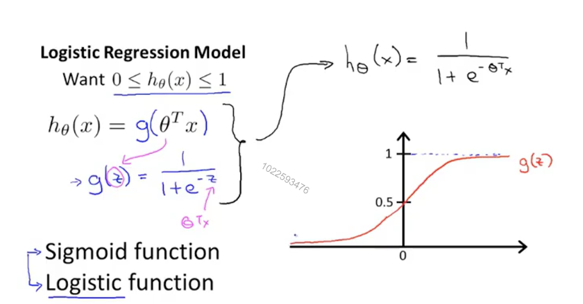
下图为Logisitic回归的假设函数,可以看出他是一个增函数,并且值区间为0~1开区间,符合我们得要求。如果最终得出值为0.7,我们可以说有70%得概率为恶心肿瘤。
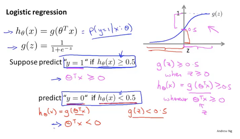
(3)决策边界:通过上面得图可以看出,当值小于0.5时判定为良性,大于0.5时判定为恶性。当函数值为0.5时,h(x)为0。也就是说h(x)大于0时判定为恶性,小于0时判定为良性(这里的h(x)就是之前线性回归的假设函数,就是theta * X)。这个边界值称为决策边界。
(4)代价函数:之前的代价函数并不是个凸函数,有很个局部最优解。用梯度下降的时候,选择不同的起始点可能得到不同的最优解。
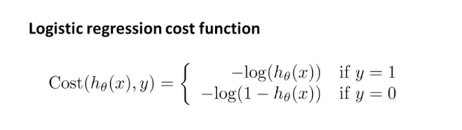
h(x)值域为0~1,所以两种情况的作用域都是0~1。y=1时是单调递减,在h(x)为1时趋近于0,h(x)为0时趋近于正无穷;y=0时单调递增,与上面相反。如果预测错误则返回一个很大的代价值用于惩罚。
为了方便计算要把两个结合到一起: - [y * (log(h(x))) + (1 - y) * log(1 - h(x))]
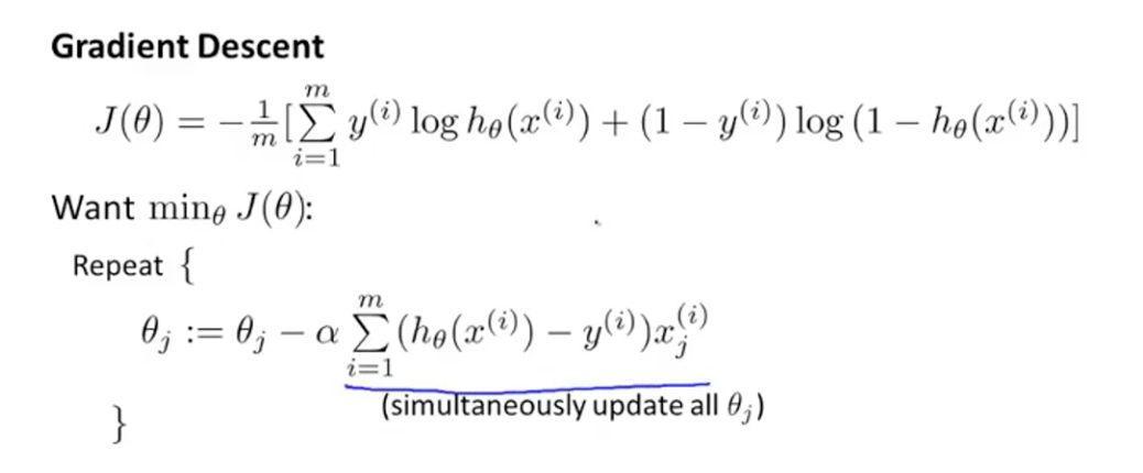
(5)求偏导之后
(6)代码:梯度下降之前也要进行特征缩放
  1 #coding=utf-8
  2 from sklearn.linear_model import LogisticRegression
  3 import matplotlib.pyplot as plt
  4 import numpy as np
  5 import math
  6 import copy
  7 np.set_printoptions(suppress=True)
  8
  9 def test(arr):
 10     res = 0
 11     for i in arr:
 12         res += math.fabs(i)
 13     return res
 14
 15
 16
 17 #读取文件
 18 def readDate(path):
 19     x_data = []
 20     y_data = []
 21     fd = open(path, 'r')
 22     for line in fd.readlines():
 23         lineArr = line.strip().split()
 24         x_data.append([1, lineArr[0], lineArr[1]])
 25         y_data.append([lineArr[2]])
 26
 27     x_data = np.array(x_data).astype(np.float)
 28     y_data = np.array(y_data).astype(np.float)
 29     return x_data, y_data
 30
 31 #sigmoid
 32 def h(x_data, p):
 33     plus = np.dot(x_data, p)
 34     for i in range(len(plus)):
 35         plus[i][0] = 1 / (1 + math.exp(-plus[i][0]))
 36     return plus
 37
 38 #特征缩放
 39 def scale(arr):
 40     param = []
 41     for i in range(1, arr.shape[1]):
 42         col = arr[:,i]
 43         mean = np.mean(col)
 44         std = np.std(col)
 45
 46         std = 1 if std == 0 else std
 47         param.insert(i, {'mean':mean, 'std':std})
 48         for j in range(0, len(col)):
 49             arr[j][i] = (col[j] - mean) / std
 50     return arr, param
 51
 52
 53
 54 def J(x_data, y_data, p, a):
 55     global m
 56     sub = h(x_data, p) - y_data
 57     deviation = np.dot(x_data.T, sub)
 58     return a / m * deviation
 59
 60 #整理参数
 61 def build(p, param):
 62     f = 1       #常数项
 63     for i in range(1, len(p)):
 64         f -= param[i - 1]['mean'] / param[i - 1]['std'] * p[i][0]
 65         p[i] = format(p[i][0] / param[i - 1]['std'], '0.2f')
 66
 67     p[0] = format(f + p[0][0], '0.2f')
 68     return p
 69
 70
 71 #画图
 72 def plotPoint(x_data, y_data, p):
 73     xcordt = []
 74     ycordt = []
 75     xcordf = []
 76     ycordf = []
 77     n = len(y_data)
 78     for i in range(n):
 79         if int(y_data[i][0]) == 1:
 80             xcordt.append(x_data[i,1])
 81             ycordt.append(x_data[i,2])
 82         else:
 83             xcordf.append(x_data[i, 1])
 84             ycordf.append(x_data[i, 2])
 85
 86     fig = plt.figure()
 87     ax = fig.add_subplot(111)
 88     ax.scatter(xcordt, ycordt, s=30, c='red', marker='s')
 89     ax.scatter(xcordf, ycordf, s=30, c='green')
 90
 91     #函数曲线
 92     x = np.arange(-3, 3, 0.1)
 93     y = -(p[0][0] + p[1][0] * x) / p[2][0]
 94     ax.plot(x,y)
 95     plt.show()
 96
 97
 98 if __name__  == '__main__':
 99     path = 'testSet.txt'
100     a = 0.5
101     x_data, y_data = readDate(path)
102     x_bak = copy.deepcopy(x_data)
103     x_data, param = scale(x_data)
104
105     m = len(x_data)
106     p = np.zeros([len(x_data[0]), 1])
107
108     step = 2000
109     for i in range(step):
110         j = J(x_data, y_data, p, a)
111         p -= j
112
113
114     p = build(p, param)
115     plotPoint(x_bak, y_data, p)