编程作业ex1:线性回归

一、热身练习

要求：生成一个5*5的单位矩阵

warmUpExercies 函数:

function A = warmUpExercise() %定义函数A为warmupexercise
A = eye(5);         %eye()单位矩阵，该函数的功能即生成5*5的单位矩阵
end

调用：

fprintf('Running warmUpExercise ... 
');
fprintf('5x5 Identity Matrix: 
');
warmUpExercise()    %调用该函数

fprintf('Program paused. Press enter to continue.
');
pause;

输出：

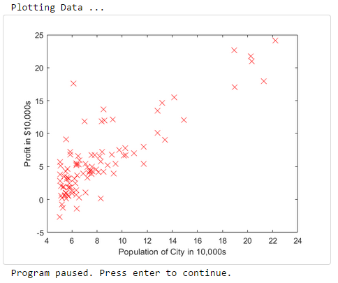
 二、绘图（plotting）

要求：根据给出的数据（第一列为所在城市的人口，第二列为对应城市的利润，负数表示亏损）绘制散点图，以更好选择餐馆的地址

plotData函数：

function plotData(x, y)
plot(x,y,'rx','MarkerSize',10);
ylabel('Profit in $10,000s');   % 设置y轴标签
xlabel('Population of City in 10,000s');  % 设置x轴标签
end

*MarkerSize: 标记大小，默认为6

* rx：红色的叉号

调用：

fprintf('Plotting Data ...
')
data = load('ex1data1.txt');    % 加载data文件
X = data(:, 1); y = data(:, 2);  % 将第一列全部元素赋值给X，第二列全部元素赋值给y
m = length(y); % 定义m为训练样本的数量

plotData(X, y);  % 将X，y作为参数调用plotData函数

fprintf('Program paused. Press enter to continue.
');
pause;

输出：

三、代价函数和梯度下降

线性回归的目标是最小化代价函数J(θ):

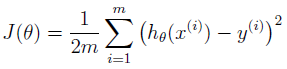 ，在这里使用平方法来表示误差，误差越小代表拟合的越好。

其中假设 h(x) 由线性模型给出:

 模型的参数是θ_j 通过调整θ的值来最小化成本函数，一种方法是梯度下降，在这种算法中，每次迭代都要更新θ

 随着梯度下降的每一步，参数θ_j 接近实现最低成本J(θ)的最佳θ值

*与 = 不同，:= 代表着 同时更新(simultaneously update)，简单来说就是先将计算的 θ存入一个临时变量，最后所有 θ都计算完了一起再赋值回去，例如

temp1 = theta1 - （theta1 - 10 * theta2 * x1） ;
temp2 = theta2 - （theta1 - 10 * theta2 * x2） ;
theta1 = temp1 ;
theta2 = temp2 ;

在数据中增加一列1，因为代价函数中θ0的系数为1，且将参数初始化为0，将学习率α初始化为0.01

矩阵表示的话类似于：

X = [ones(m, 1), data(:,1)];  % 向x第一列添加一列1
theta = zeros(2, 1); % 初始化拟合参数

iterations = 1500;   % 迭代次数
alpha = 0.01;    % 学习率设置为0.01

 ==》计算代价函数J（检测收敛性）

function J = computeCost(X, y, theta)
m = length(y);
J = 0;
J = sum((X*theta-y).^2)/(2*m);
end

调用代价函数：

fprintf('
Testing the cost function ...
')
% compute and display initial cost 
J = computeCost(X, y, theta);  % 调用代价函数J
fprintf('With theta = [0 ; 0]
Cost computed = %f
', J);
fprintf('Expected cost value (approx) 32.07
');

% further testing of the cost function
J = computeCost(X, y, [-1 ; 2]);  % 调用代价函数J

fprintf('
With theta = [-1 ; 2]
Cost computed = %f
', J); 
fprintf('Expected cost value (approx) 54.24
'); 
fprintf('Program paused. Press enter to continue.
'); 
pause;

运行结果：

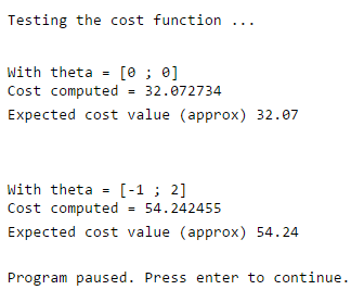
 可以看到，当theta取[0;0]时的代价函数比取[-1;2]的代价函数小，说明[0;0]更优。

gradientDescent.m——运行梯度下降：

说明：验证梯度下降是否正常工作的一种好方法是查看J的值并检查它是否随每一步减少。 gradientDescent.m的代码在每次迭代时调用computeCost并打印J的值。 假设已正确实现了梯度下降和computeCost，则J的值不应该增加，并且应该在算法结束时收敛到稳定值。

在梯度下降中，每次迭代都执行下面的这个更新：

梯度下降函数：

function [theta, J_history] = gradientDescent(X, y, theta, alpha, num_iters)
%GRADIENTDESCENT Performs gradient descent to learn theta
%   theta = GRADIENTDESCENT(X, y, theta, alpha, num_iters) updates theta by 
%   taking num_iters gradient steps with learning rate alpha

% Initialize some useful values
m = length(y); % number of training examples
J_history = zeros(num_iters, 1);

for iter = 1:num_iters

    % ====================== YOUR CODE HERE ======================
    % Instructions: Perform a single gradient step on the parameter vector
    %               theta. 
    %
    % Hint: While debugging, it can be useful to print out the values
    %       of the cost function (computeCost) and gradient here.
    %

    theta = theta-alpha*(1/m)*X'*(X*theta-y);

    % ============================================================

    % Save the cost J in every iteration    
    J_history(iter) = computeCost(X, y, theta);

end

end

 调用梯度下降函数：

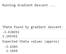
fprintf('
Running Gradient Descent ...
')
% run gradient descent  运行梯度下降函数
theta = gradientDescent(X, y, theta, alpha, iterations);

% print theta to screen 将theta值输出
fprintf('Theta found by gradient descent:
');  % 利用梯度下降函数计算出的theta
fprintf('%f
', theta);
fprintf('Expected theta values (approx)
');  % 期望的theta
fprintf(' -3.6303
  1.1664

');

运行结果：

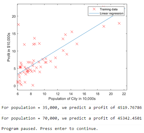
 将得到的参数用MATLAB进行绘制并预测35000和70000人口的利润：

% Plot the linear fit 绘制线性拟合直线
hold on; % keep previous plot visible  指当前图形保持，即样本点仍然保持在图像上
plot(X(:,2), X*theta, '-')
legend('Training data', 'Linear regression') % 创建图例标签
hold off % don't overlay any more plots on this figure

% Predict values for population sizes of 35,000 and 70,000
predict1 = [1, 3.5] *theta;
fprintf('For population = 35,000, we predict a profit of %f
',...
    predict1*10000);
predict2 = [1, 7] * theta;
fprintf('For population = 70,000, we predict a profit of %f
',...
    predict2*10000);

fprintf('Program paused. Press enter to continue.
');
pause;

运行结果：

 *注意A*B和A.*B的区别，前者进行矩阵乘法，后者进行逐元素乘法

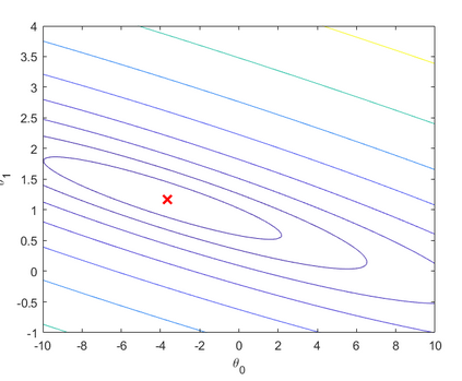
四、可视化代价函数J

这部分代码已经给出

fprintf('Visualizing J(theta_0, theta_1) ...
')

% Grid over which we will calculate J
theta0_vals = linspace(-10, 10, 100);
theta1_vals = linspace(-1, 4, 100);

% initialize J_vals to a matrix of 0's
J_vals = zeros(length(theta0_vals), length(theta1_vals));

% Fill out J_vals
for i = 1:length(theta0_vals)
    for j = 1:length(theta1_vals)
      t = [theta0_vals(i); theta1_vals(j)];
      J_vals(i,j) = computeCost(X, y, t);
    end
end


% Because of the way meshgrids work in the surf command, we need to
% transpose J_vals before calling surf, or else the axes will be flipped
J_vals = J_vals';
% Surface plot
figure;
surf(theta0_vals, theta1_vals, J_vals)
xlabel('	heta_0'); ylabel('	heta_1');

% Contour plot
figure;
% Plot J_vals as 15 contours spaced logarithmically between 0.01 and 100
contour(theta0_vals, theta1_vals, J_vals, logspace(-2, 3, 20))
xlabel('	heta_0'); ylabel('	heta_1');
hold on;
plot(theta(1), theta(2), 'rx', 'MarkerSize', 10, 'LineWidth', 2);

运行结果：