(一)K近邻算法基础
K近邻(KNN)算法优点
- 思想极度简单
- 应用数学知识少(近乎为0)
- 效果好
- 可以解释机器学习算法使用过程中的很多细节问题
- 更完整的刻画机器学习应用的流程
图解K近邻算法

上图是以往病人体内的肿瘤状况,红色是良性肿瘤、蓝色是恶性肿瘤。显然这与发现时间的早晚以及肿瘤大小有密不可分的关系,那么当再来一个病人,我怎么根据时间的早晚以及肿瘤大小推断出这个新的病人体内的肿瘤(图中的绿色)是良性的还是恶性的呢?
k近邻的思想便可以在这里使用,我根据距离(至于距离是什么样的距离,我们后面会说,目前就以图上看到的)选择离其最近的K个,这里K取3,那么就看离自己最近的3个肿瘤。看看其标签,哪个出现的次数最多。这里三个都是蓝色(恶性),蓝色比红色等于3比0,蓝色出现的次数最多,那么我们通过k近邻算法就可以说这个肿瘤是恶性的。
因此K近邻思想,还是看样本的相似度。数量取得过少则具备偶然性,所以多取几个,看看K个里面出现最多的样本的标签。
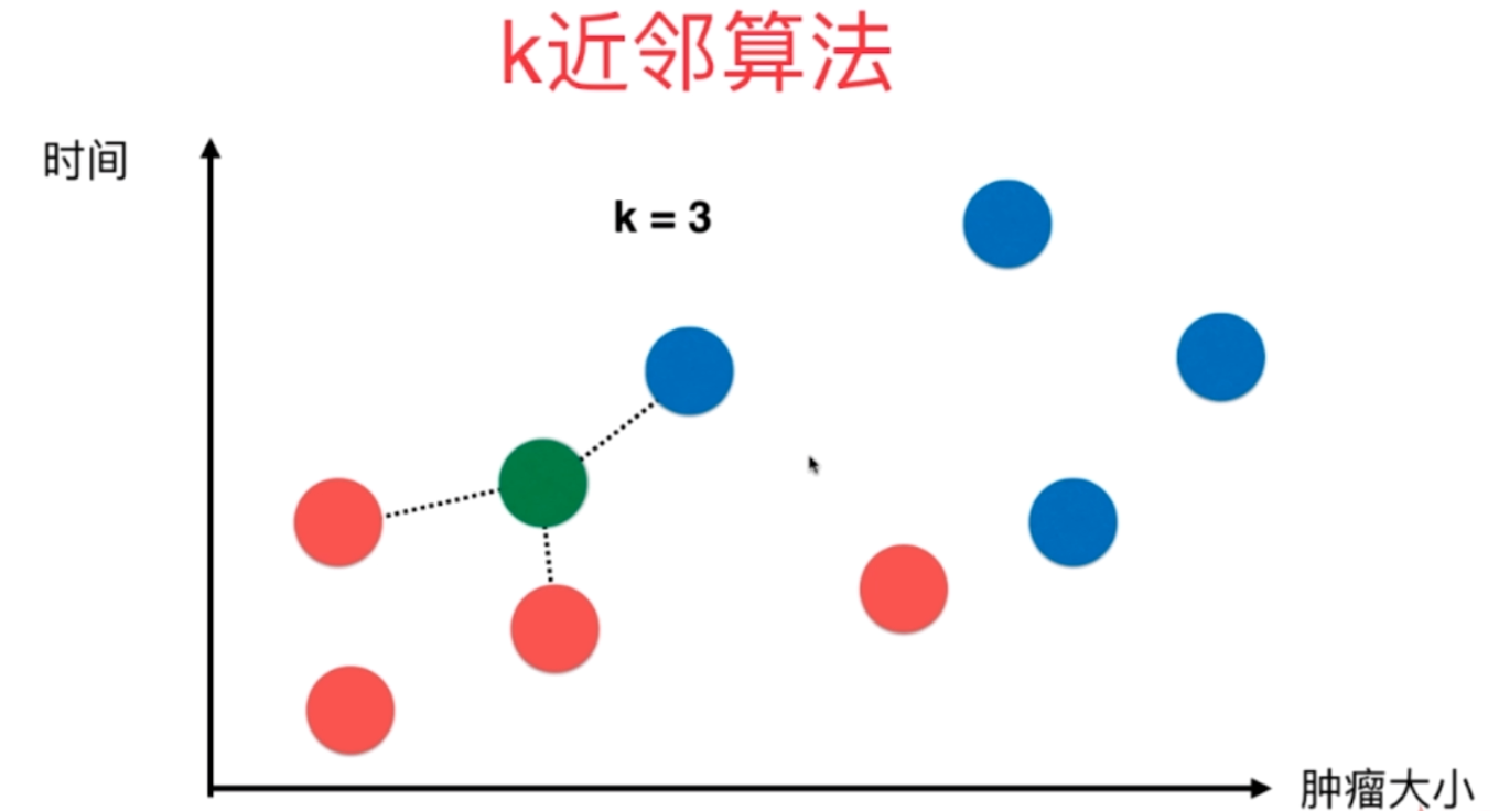
当再来一个肿瘤的时候,此时红色比蓝色等于2比1,红色胜出。那么K近邻就告诉我们,这个肿瘤很可能是一个良性肿瘤。
K近邻代码实现
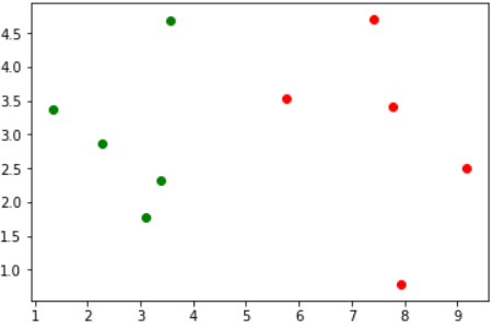
先来看看数据集
import numpy as np
import matplotlib.pyplot as plt

# 可以看做肿瘤的发现时间和大小
raw_data_X = [[3.39, 2.33],
              [3.11, 1.78],
              [1.34, 3.37],
              [3.58, 4.68],
              [2.28, 2.87],
              [7.42, 4.70],
              [5.75, 3.53],
              [9.17, 2.51],
              [7.79, 3.42],
              [7.94, 0.79]]

# 可以看做是良性还是恶性
raw_date_y = [0, 0, 0, 0, 0, 1, 1, 1, 1, 1]

# 这里都当做训练集
X_train = np.array(raw_data_X)
y_train = np.array(raw_date_y)

# 选择标签为0所对应的样本
plt.scatter(X_train[y_train == 0, 0], X_train[y_train == 0, 1], color="green")
# 选择标签为1所对应的样本
plt.scatter(X_train[y_train == 1, 0], X_train[y_train == 1, 1], color="red")
plt.show()
运行结果
当我再来一个数据的时候
x = np.array([8.09, 3.37])
plt.scatter(X_train[y_train == 0, 0], X_train[y_train == 0, 1], color="green")
plt.scatter(X_train[y_train == 1, 0], X_train[y_train == 1, 1], color="red")
# 我们将这个点也进行绘制,使用不同的颜色
plt.scatter(x[0], x[1], color="blue")
plt.show()
运行结果
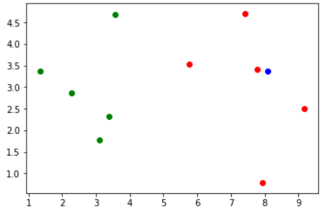
根据图像我们可以看出,这个新来的数据(蓝色)应该是属于红色这一类的。那么下面我们就整体通过代码来实现一下。
import numpy as np


raw_data_X = [[3.39, 2.33],
              [3.11, 1.78],
              [1.34, 3.37],
              [3.58, 4.68],
              [2.28, 2.87],
              [7.42, 4.70],
              [5.75, 3.53],
              [9.17, 2.51],
              [7.79, 3.42],
              [7.94, 0.79]]

raw_date_y = [0, 0, 0, 0, 0, 1, 1, 1, 1, 1]

X_train = np.array(raw_data_X)
y_train = np.array(raw_date_y)
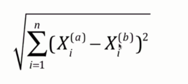
接下来计算图中每一个点与新来的点的距离,关于距离的计算我们选择欧拉距离
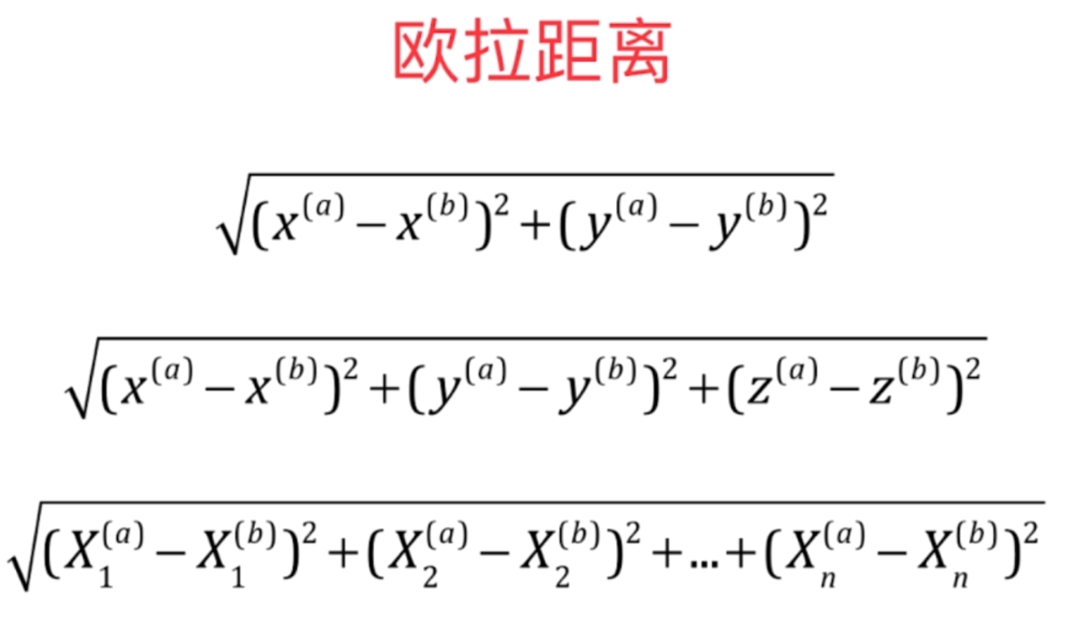
就是将每一个特征相减再平方,然后相加、开根号
简化一下表示就是这样
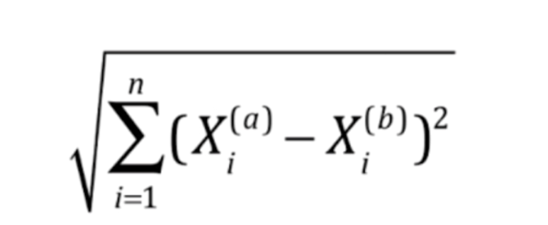
将a样本和b样本的第i个特征进行相减,然后平方,求和,整体开根号
x = np.array([8.09, 3.37])  # 新来的点
distances = []  # 用于存放图中每一个点和新来的点的距离
for x_train in X_train:
    d = np.sqrt(np.sum( (x_train - x) ** 2 ))
    distances.append(d)

# 先来看看distances
print(distances)
运行结果
[4.813688814204756,
 5.227666783566069,
 6.75,
 4.696402878799901,
 5.831474942070831,
 1.4892279879185726,
 2.3454637068179074,
 1.3805795884337855,
 0.3041381265149108,
 2.584356786513813]
我们得到了每个点与新来的点之间的距离,那么我们可以进行排序,注意:是按照值得大小来对索引进行排序
nearest = np.argsort(distances)
print(nearest)
运行结果
[8 7 5 6 9 3 0 1 4 2]
表示离自己最近的,在原来索引为8的位置,第二近的为索引为7的位置。
# 选择离自己最近的K个样本
k = 6
topK_y = y_train[nearest[: k]]
print(topK_y)
from collections import Counter
# 进行投票,选择出现次数最多的那个元素
votes = Counter(topK_y).most_common(1)[0]
print(f"标签{votes[0]}出现次数最多,出现{votes[1]}次")
运行结果
[1 1 1 1 1 0]
标签1出现次数最多,出现5次
以上便是我们简单地使用K近邻算法对样本数据进行的一个简单的预测
(二)sklearn中的机器学习算法封装
简单的自定义
import numpy as np
from collections import Counter


def knn_classify(k, X_train, y_train, x):
    """
    :param k: k近邻的那个k
    :param X_train: 训练样本
    :param y_train: 标签
    :param x: 预测样本
    :return:
    """
    assert 1 <= k <= X_train.shape[0], "K必须大于等于1,并且小于等于训练样本的总数量"
    assert X_train.shape[0] == y_train.shape[0], "训练样本的数量必须和标签数量保持一致"
    assert x.shape[0] == X_train.shape[1], "预测样本的特征数必须和训练样本的特征数保持一致"

    distances = [np.sqrt(np.sum((x_train - x) ** 2)) for x_train in X_train]
    nearest = np.argsort(distances)

    topK_y = y_train[nearest[: k]]
    votes = Counter(topK_y).most_common(1)[0]

    return f"该样本的特征为{votes[0]},在{k}个样本中出现了{votes[1]}次"


raw_data_X = [[3.39, 2.33],
              [3.11, 1.78],
              [1.34, 3.37],
              [3.58, 4.68],
              [2.28, 2.87],
              [7.42, 4.70],
              [5.75, 3.53],
              [9.17, 2.51],
              [7.79, 3.42],
              [7.94, 0.79]]

raw_date_y = [0, 0, 0, 0, 0, 1, 1, 1, 1, 1]

X_train = np.array(raw_data_X)
y_train = np.array(raw_date_y)
x = np.array([8.09, 3.37])  # 新来的点

print(knn_classify(3, X_train, y_train, x))
运行结果
该样本的特征为1,在3个样本中出现了3次
什么是机器学习
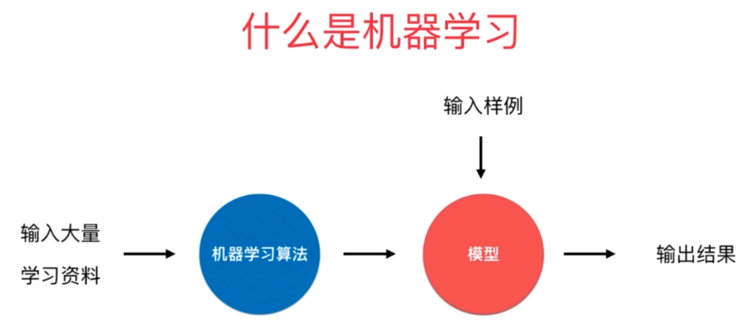
k近邻算法是一种机器学习算法,那么机器学习是什么呢?机器学习就是我们输入大量的学习资料,然后通过机器学习算法(k近邻只是其中一种)训练出一个模型,当下一个样例到来的时候,我们预测出结果。
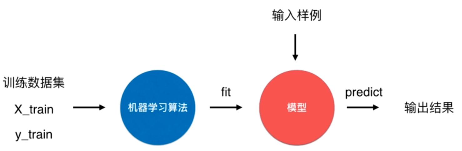
我们输入的与其说是学习资料,倒不如说是样本(训练数据集),这个样本里面包含了X_train(样本特征)和y_train(样本标签),通过机器学习算法,对样本进行训练得到模型(特征和标签之间的对应关系)这一过程我们称之为fit(拟合),然后输入新的样本根据上一步得到的模型来预测出结果这一过程我们称之为predict(预测)
可是我们在k近邻算法中,并没有看到训练模型这一步啊,可以这么说,k近邻是一个不需要训练过程的算法。
k近邻算法是非常特殊的,可以认为没有模型的算法。为了和其他算法统一,可以认为训练数据集本身就是模型。
因此我们还是为k近邻找到了一个fit的过程,这在sklearn中也是这么设计的。sklearn里面封装了大量的算法,它们的设计理念都是一样的,都是先fit训练模型,然后predict进行预测。
sklearn中的k近邻算法
import numpy as np
from sklearn.neighbors import KNeighborsClassifier


# sklearn里面所有的算法都是以面向对象的形式封装的
knn = KNeighborsClassifier(n_neighbors=3)  # 这里的n_neighbors就是knn的那个k
# fit
raw_data_X = [[3.39, 2.33],
              [3.11, 1.78],
              [1.34, 3.37],
              [3.58, 4.68],
              [2.28, 2.87],
              [7.42, 4.70],
              [5.75, 3.53],
              [9.17, 2.51],
              [7.79, 3.42],
              [7.94, 0.79]]

raw_date_y = [0, 0, 0, 0, 0, 1, 1, 1, 1, 1]

X_train = np.array(raw_data_X)
y_train = np.array(raw_date_y)
knn.fit(X_train, y_train)
# predict
y_predict = knn.predict(np.array([[8.09, 3.37],
                                  [3.09, 7.37]]))
# 在sklearn中,predict必须要传递一个二维数组, 哪怕只有一个元素,也要写成二维数组的模式

print(y_predict)
运行结果
[1 0]
总结一下就是:
- 每个算法在sklearn中就是一个类,通过给类指定参数(不指定会用默认的)得到一个实例
- 调用实例的fit方法,传入训练数据集的特征和标签,来训练出一个模型。并且这个方法会返回实例本身,我们不需要再单独的接收
- fit完毕之后,直接调用predict,得到预测的结果。并且注意的是,在sklearn中,要传入二维数组,哪怕只预测一个样本也要以二维数组的形式传递。比如:np.array([8.09, 3.37]),要传递np.array([[8.09, 3.37]])
- 保存得到的预测值
在sklearn中所有的算法都保持者这样的高度一致性,都是得到实例,再fit,然后predict
封装自己的knn
显然以这种类的模式,是更加友好的。那么我们也可以将我们之间写的knn算法,封装成sklearn中knn的模式
import numpy as np
from collections import Counter


class KnnClassifier:

    def __init__(self, k):
        assert k >= 1, "K必须合法"
        self.k = k
        # 用户肯定会传入样本集,因此提前写好。使用私有变量表示这些变量不建议从外部访问。
        self._X_train = None
        self._y_train = None

    def fit(self, X_train, y_train):
        assert X_train.shape[0] == y_train.shape[0], "训练样本的数量必须和标签数量保持一致"
        assert self.k <= X_train.shape[0], "K必须小于等于训练样本的总数量"
        self._X_train = X_train
        self._y_train = y_train

        return self
        # 这里完全可以不需要return self,但是为了和sklearn中的格式保持一致,我们还是加上这句
        # 为什么这么做呢?其实如果我们严格按照sklearn的标准来写的话,那么我们自己写的算法是可以和sklearn中的其他算法无缝对接的

    def predict(self, X_predict):
        assert self._X_train is not None and self._y_train is not None, "在predict之间必须先进行fit"
        if not isinstance(X_predict, np.ndarray):
            raise TypeError("传入的数据集必须是np.ndarray类型")

        predict = []
        # 因为可能来的不止一个样本
        for x in X_predict:
            distances = [np.sqrt(np.sum((x_train - x) ** 2)) for x_train in self._X_train]
            nearest = np.argsort(distances)

            votes = self._y_train[nearest[: self.k]]
            predict.append(Counter(votes).most_common(1)[0][0])

        # 遵循sklearn的标准,以np.ndarry的形式返回
        return np.array(predict)

    def __repr__(self):
        return f"KNN(k={self.k})"

    def __str__(self):
        return f"KNN(k={self.k})"


raw_data_X = [[3.39, 2.33],
              [3.11, 1.78],
              [1.34, 3.37],
              [3.58, 4.68],
              [2.28, 2.87],
              [7.42, 4.70],
              [5.75, 3.53],
              [9.17, 2.51],
              [7.79, 3.42],
              [7.94, 0.79]]

raw_date_y = [0, 0, 0, 0, 0, 1, 1, 1, 1, 1]

X_train = np.array(raw_data_X)
y_train = np.array(raw_date_y)
x = np.array([[8.09, 3.37],
              [5.75, 3.53]])  # 新来的点

knn = KnnClassifier(k=3)
knn.fit(X_train, y_train)
print(knn)
y_predict = knn.predict(x)

print(y_predict)
运行结果
KNN(k=3)
[1 1]
(三)训练数据集、测试数据集
判断机器学习算法的性能
我们通过训练得到模型,可以我们是将所有的训练数据集都拿来训练模型。

如果模型很差怎么办?我们没有机会去调整,因为我们的模型是要在真实的环境中使用的。
因此这种方式,我们无法得知模型的好坏,在真实的环境中使用就只能听天由命了。
说了这么多,意思就是将全部的数据集都用来寻来模型是不合适的,因此我们可以将数据集进行分割。比如百分之80的数据集用来训练,百分之20的数据集用于测试

如果对测试数据集预测的不够好的话,说明我们的算法还需要改进,这样就可以在进入真实环境之前改进模型。
这个过程我们称之为train test split,训练测试数据集进行分割。

将我们之前自己写的knn算法和切割数据集的代码组合起来,一部分用于训练,一部分用于预测
import numpy as np
from collections import Counter
from sklearn.datasets import load_iris


class KnnClassifier:

    def __init__(self, k):
        assert k >= 1, "K必须合法"
        self.k = k
        # 用户肯定会传入样本集,因此提前写好。使用私有变量表示这些变量不建议从外部访问。
        self._X_train = None
        self._y_train = None

    def fit(self, X_train, y_train):
        assert X_train.shape[0] == y_train.shape[0], "训练样本的数量必须和标签数量保持一致"
        assert self.k <= X_train.shape[0], "K必须小于等于训练样本的总数量"
        self._X_train = X_train
        self._y_train = y_train

        return self
        # 这里完全可以不需要return self,但是为了和sklearn中的格式保持一致,我们还是加上这句
        # 为什么这么做呢?其实如果我们严格按照sklearn的标准来写的话,那么我们自己写的算法是可以和sklearn中的其他算法无缝对接的

    def predict(self, X_predict):
        assert self._X_train is not None and self._y_train is not None, "在predict之间必须先进行fit"
        if not isinstance(X_predict, np.ndarray):
            raise TypeError("传入的数据集必须是np.ndarray类型")

        predict = []
        # 因为可能来的不止一个样本
        for x in X_predict:
            distances = [np.sqrt(np.sum((x_train - x) ** 2)) for x_train in self._X_train]
            nearest = np.argsort(distances)

            votes = self._y_train[nearest[: self.k]]
            predict.append(Counter(votes).most_common(1)[0][0])

        # 遵循sklearn的标准,以np.ndarry的形式返回
        return np.array(predict)

    def __repr__(self):
        return f"KNN(k={self.k})"

    def __str__(self):
        return f"KNN(k={self.k})"


def train_test_split(X, y, test_size=0.3):
    """
    :param X: 训练样本
    :param y: 特征
    :param test_size: 测试集所占的比例
    :return:
    """
    # 根据数据集的个数生成相应数量的索引
    index = np.arange(X.shape[0])
    # 将索引打乱
    np.random.shuffle(index)
    # 150个样本,乘上0.3等于45
    train_count = index[int(X.shape[0] * test_size):]  # [45: ]
    test_count = index[: int(X.shape[0] * test_size)]  # [: 45]

    X_train = X[train_count]
    y_train = y[train_count]
    X_test = X[test_count]
    y_test = y[test_count]
    return X_train, y_train, X_test, y_test


knn = KnnClassifier(k=5)
iris = load_iris()
X = iris.data
y = iris.target

X_train, y_train, X_test, y_test = train_test_split(X, y, test_size=0.3)
knn.fit(X_train, y_train)
# 预测
y_predict = knn.predict(X_test)
# 将对测试集进行预测的结果和已知的结果进行比对
print(f"测试样本总数:{len(X_test)}, "
      f"预测正确的数量:{np.sum(y_predict == y_test)}, "
      f"预测准确率:{np.sum(y_predict == y_test) / len(X_test)}")
运行结果
测试样本总数:45, 预测正确的数量:44, 预测准确率:0.9777777777777777
可以看到,预测结果还是不错的。
sklearn中train_test_split
from sklearn.model_selection import train_test_split
X_train, X_test, y_train, y_test = train_test_split(X, y, test_size=0.3)
可以看到我们之前设计的train_test_split和sklearn中train_test_split接口是一致的,只是我们自己实现的train_test_split的返回值顺序貌似写错了。不过无所谓,只要返回值顺序和我们接收的顺序一样就行,在下面的例子会改正过来。而且sklearn中可以接收更多的参数,比如我们还可以设置一个random_state,表示随机种子。
因此以上就是训练集和测试集的内容,训练集进行训练,测试集进行测试。如果在测试集上表现完美的话,我们才会投入生产环境使用,如果表现不完美,那么我们可能就要调整我们的算法,或者调整我们的参数了
(四)分类准确度
评价一个算法的好坏,我们可以使用分类准确度来实现。如果预测正确的样本个数越多,那么说明我们的算法越好
metrics.py
import numpy as np


def accuracy_score(y_true, y_predict):

    assert y_true.shape == y_predict.shape, "预测值和真实值的个数必须一致"
    return np.sum(y_true == y_predict) / len(y_true)
model_selection.py
import numpy as np


def train_test_split(X, y, test_size=0.3):
    index = np.arange(X.shape[0])
    np.random.shuffle(index)
    train_count = index[int(X.shape[0] * test_size):]
    test_count = index[: int(X.shape[0] * test_size)]

    X_train = X[train_count]
    y_train = y[train_count]
    X_test = X[test_count]
    y_test = y[test_count]

    return X_train, X_test, y_train, y_test
knn.py
import numpy as np
from collections import Counter


class KnnClassifier:

    def __init__(self, k):
        assert k >= 1, "K必须合法"
        self.k = k
        self._X_train = None
        self._y_train = None

    def fit(self, X_train, y_train):
        assert X_train.shape[0] == y_train.shape[0], "训练样本的数量必须和标签数量保持一致"
        assert self.k <= X_train.shape[0], "K必须小于等于训练样本的总数量"
        self._X_train = X_train
        self._y_train = y_train

        return self

    def predict(self, X_predict):
        assert self._X_train is not None and self._y_train is not None, "在predict之间必须先进行fit"
        if not isinstance(X_predict, np.ndarray):
            raise TypeError("传入的数据集必须是np.ndarray类型")

        predict = []
        for x in X_predict:
            distances = [np.sqrt(np.sum((x_train - x) ** 2)) for x_train in self._X_train]
            nearest = np.argsort(distances)

            votes = self._y_train[nearest[: self.k]]
            predict.append(Counter(votes).most_common(1)[0][0])

        return np.array(predict)

    def __repr__(self):
        return f"KNN(k={self.k})"

    def __str__(self):
        return f"KNN(k={self.k})"
from sklearn.datasets import load_digits
from model_selection import train_test_split
from knn import KnnClassifier
from metrics import accuracy_score


# 使用sklearn中的手写字体
digits = load_digits()
X = digits.data
print(X.shape)
"""
(1797, 64)
说明总共有1797个样本,每个样本都有64个特征
"""
y = digits.target
print(y.shape)
"""
(1797,)
"""
print(digits.target_names)
"""
[0 1 2 3 4 5 6 7 8 9]
"""

X_train, X_test, y_train, y_test = train_test_split(X, y, test_size=0.3)
k = KnnClassifier(k=3)
k.fit(X_train, y_train)
y_predict = k.predict(X_test)

print(accuracy_score(y_test, y_predict))  # 0.9851576994434137
分类的结果还是比较准确的。
有些时候我们之所以得到预测值,其实还是为了将预测值和真实值进行对比,从而得到准确率,那么我们也可以在算法中封装一个类似的功能。
knn.py
import numpy as np
from collections import Counter
from metrics import accuracy_score


class KnnClassifier:

    def __init__(self, k):
        assert k >= 1, "K必须合法"
        self.k = k
        self._X_train = None
        self._y_train = None

    def fit(self, X_train, y_train):
        assert X_train.shape[0] == y_train.shape[0], "训练样本的数量必须和标签数量保持一致"
        assert self.k <= X_train.shape[0], "K必须小于等于训练样本的总数量"
        self._X_train = X_train
        self._y_train = y_train

        return self

    def predict(self, X_predict):
        assert self._X_train is not None and self._y_train is not None, "在predict之间必须先进行fit"
        if not isinstance(X_predict, np.ndarray):
            raise TypeError("传入的数据集必须是np.ndarray类型")

        predict = [self.__predict(x) for x in X_predict]

        return np.array(predict)

    def __predict(self, x):
        distances = [np.sqrt(np.sum((x_train - x) ** 2)) for x_train in self._X_train]
        nearest = np.argsort(distances)

        votes = self._y_train[nearest[: self.k]]
        return Counter(votes).most_common(1)[0][0]

    def score(self, X_test, y_test):
        y_predict = self.predict(X_test)
        return accuracy_socre(y_test, y_predict)

    def __repr__(self):
        return f"KNN(k={self.k})"

    def __str__(self):
        return f"KNN(k={self.k})"
from sklearn.datasets import load_digits
from model_selection import train_test_split
from knn import KnnClassifier


digits = load_digits()
X = digits.data
y = digits.target

X_train, X_test, y_train, y_test = train_test_split(X, y, test_size=0.3)
k = KnnClassifier(k=3)
k.fit(X_train, y_train)

print(k.score(X_test, y_test))  # 0.9888682745825603
这样我们就实现了直接传入测试集就能计算准确度的方法,不需要再手动计算predict,同样这和sklearn中的接口也是保持一致的。
下面来看看sklearn中的accuracy_score
from sklearn.datasets import load_digits
from sklearn.model_selection import train_test_split
from sklearn.neighbors import KNeighborsClassifier
from sklearn.metrics import accuracy_score


digits = load_digits()
X = digits.data
y = digits.target

X_train, X_test, y_train, y_test = train_test_split(X, y, test_size=0.3)
k = KNeighborsClassifier(n_neighbors=3)
k.fit(X_train, y_train)
y_predict = k.predict(X_test)

print(accuracy_score(y_test, y_predict))  # 0.987037037037037
同理sklearn中也封装了score这个方法
from sklearn.datasets import load_digits
from sklearn.model_selection import train_test_split
from sklearn.neighbors import KNeighborsClassifier


digits = load_digits()
X = digits.data
y = digits.target

X_train, X_test, y_train, y_test = train_test_split(X, y, test_size=0.3)
k = KNeighborsClassifier(n_neighbors=3)
k.fit(X_train, y_train)
print(k.score(X_test, y_test))  # 0.9777777777777777
# accuracy_score是我们通过X_test手动计算出y_predict,然后和y_true一起传进去进行计算
# score则不需要我们计算y_predict,而是直接传入X_test和y_test,会自动进行计算y_predict然后和y_true进行计算。
# 可以把score看成是 计算y_predict,和accuracy_score两步之和
因此如果不需要y_predict,只要看准确率的话,可以使用score
(五)超参数
之前我们在生成实例的时候,比如KNeighborsClassifier(),我们并没有指定参数。而是使用默认地参数,那么这些参数有没有用呢?存在即合理,这些参数就是超参数,顾名思义就是在fit之前,需要指定的参数。比如knn中的k,就是一个典型的超参数。
超参数和模型参数
-
超参数:在算法运行前(或者说在fit之前)需要决定的参数
-
模型参数:算法过程中学习的参数
knn算法比较特殊,它没有模型参数,因为数据集本身就可以看做成一个模型。但是后续的算法中,比如线性回归算法,都会包含大量的模型参数。
knn算法中的k是典型的超参数
寻找好的超参数
在机器学习中,我们经常会听到一个词叫"调参",这个调参调的参数指的就是超参数,因为这是在算法运行前就需要指定好的参数。
那么如何寻找好的超参数呢?
-
领域知识
这个是根据所处的领域来决定的,比如文本处理,视觉领域等等,不同的领域会有不同的超参数 -
经验数值
根据以往的经验,比如sklearn的knn算法中,默认的k就是5,这个是根据经验决定的 -
实验搜索
如果无法决定的话,那么就只能通过实验来进行搜索了。我们对超参数取不同的值进行测试、对比,寻找一个最好的超参数from sklearn.datasets import load_digits from sklearn.model_selection import train_test_split from sklearn.neighbors import KNeighborsClassifier digits = load_digits() X = digits.data y = digits.target X_train, X_test, y_train, y_test = train_test_split(X, y, test_size=0.3, random_state=666) def search_best_k(): best_score = 0.0 best_k = -1 for k in range(1, 11): knn_clf = KNeighborsClassifier(n_neighbors=k) knn_clf.fit(X_train, y_train) score = knn_clf.score(X_test, y_test) if score > best_score: best_score = score best_k = k return f"the best score is {best_score}, k is {best_k}" print(search_best_k()) # the best score is 0.9888888888888889, k is 6以上便是调参的过程,通过对不同的超参数取值,确定一个最好的超参数。当然我的机器以及版本得出来的是6,可能不同的人计算之后,得到的结果会有所差异。
但是当我们得到k是10的话,这就意味着我们得到k值是处于边界,那么我们不确定边界之外的值对算法的影响如何,可能10以后的效果会更好。因此我们还需要对10以外的值进行判断,在参数值取到我们给定的范围的边界的时候,我们需要稍微地再拓展一下,扩大搜索范围,对边界之外的值进行检测、判断,看看能否得到更好的超参数。
k近邻的其他超参数
实际上,knn不止一个超参数,还有一个很重要的超参数,那就是距离。

按照我们之前讲的,在k取3的时候,蓝色有两个,红色有1个,那么蓝色比红色是2比1。但是我们忽略了一个问题,那就是距离,这个绿色是不是离红色更近一些呢?假设有些肿瘤很奇怪,一般发现时间和大小比较接近的话,那么肿瘤的性质也类似,但是大千世界无奇不有,总会有那么几个特异的。比如红色,如果绿色和红色的情况比较类似,那么它们离得又很近,理论上结果也比较相似,但是我们选择了3个,还有两个是蓝色的,但是两者都离绿色比较远。因此如果还用个数投票的话,那么显然是不公平的,因此距离近的,那么相应的权重是不是也要更大一些呢?
因此我们可以采用距离的倒数进行计算。

采用距离的倒数,还可以有一个好处,那就是解决平票的问题
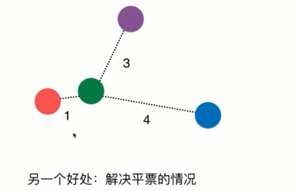
如果样本的标签有三个,但是我们k取3,那么k近邻只能随机选择一个,因此采用距离的方式,依旧可以得出红色获胜。
sklearn中knn的其他参数
__init__函数
    def __init__(self, n_neighbors=5,
                 weights='uniform', algorithm='auto', leaf_size=30,
                 p=2, metric='minkowski', metric_params=None, n_jobs=1,
                 **kwargs):

n_neighbors=5: knn当中的k,指定以几个最邻近的样本具有投票权

weights:每个拥有投票权的样本是按照什么比重投票。默认是uniform表示等比重,也就是不考虑距离,每一个成员的权重都是一样的。还可以指定为distance,就是我们之前说的按照距离的反比进行投票。

algorithm="auto": 内部采用什么样的算法实现,有以下几种方法,"ball_tree":球树,"kd_tree":kd树,"brute":暴力搜索。"auto"表示自动根据数据类型和结构选择合适的算法。一般来说,低维数据用kd_tree,高维数据用ball_tree

leaf_size=30:ball_tree或者kd_tree的叶子节点规模

matric="minkowski":怎样度量距离,默认是闵可夫斯基距离

p=2: 闵式距离各种不同的距离参数

metric_params=None:距离度量函数的额外关键字参数,一般默认为None,不用管

n_jobs=1,并行的任务数

一般来说n_neighbors、weights、p这三个参数对于调参来说是最常用的
下面我们就来考虑n_neighbors和weights这个两个参数
from sklearn.datasets import load_digits
from sklearn.model_selection import train_test_split
from sklearn.neighbors import KNeighborsClassifier


digits = load_digits()
X = digits.data
y = digits.target

X_train, X_test, y_train, y_test = train_test_split(X, y, test_size=0.3, random_state=666)


def search_best_k():
    best_weight = ""
    best_score = 0.0
    best_k = -1
    for weight in ["uniform", "distance"]:
        for k in range(1, 11):
            knn_clf = KNeighborsClassifier(n_neighbors=k, weights=weight)
            knn_clf.fit(X_train, y_train)
            score = knn_clf.score(X_test, y_test)
            if score > best_score:
                best_score = score
                best_k = k
                best_weight = weight
    return f"the best score is {best_score}, k is {best_k}, weight is {best_weight}"


print(search_best_k())  # the best score is 0.9888888888888889, k is 6, weight is uniform
这是将距离考虑进去之后的结果
更多关于距离的定义
我们之前讨论距离,显然都是欧拉距离。说白了就是两点确认一条直线,这条直线的长度。
那么下面我们介绍更多的距离,其实sklearn的knn的参数中,我们貌似看到了一个闵可夫斯基距离(闵式距离),也会在下面介绍。
- 欧拉距离
这个无需介绍,就是两个点连接的直线的距离
- 曼哈顿距离

曼哈顿距离,是在各个维度上的距离之和。也就是图中蓝色的距离,或者说是红色的距离、黄色的距离,三者都是一样的,各个维度上的距离之和就是曼哈顿距离。那么图中的绿色的那条线显然就是欧拉距离。
-
闵可夫斯基距离
首先曼哈顿距离是每个维度的距离之和
欧拉距离是每个维度的距离的平方之和再开平方
闵可夫斯基距离则是每个维度的距离的p次方之和再开p次方

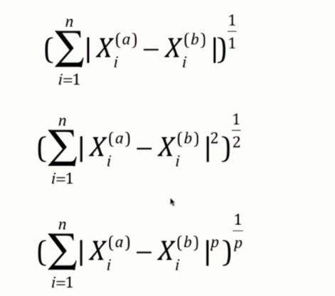
因此曼哈顿距离和欧拉距离可以看成是闵可夫斯基距离的p分别取1和2所对应的情况。
在sklearn的knn中,里面就有一个参数p,这个p指的就是图中闵式距离里面的p。而p默认取2,那么显然默认就是欧拉距离。
搜索最好的参数p
from sklearn.datasets import load_digits
from sklearn.model_selection import train_test_split
from sklearn.neighbors import KNeighborsClassifier


digits = load_digits()
X = digits.data
y = digits.target

X_train, X_test, y_train, y_test = train_test_split(X, y, test_size=0.3, random_state=666)


def search_best_k():
    best_p = -1
    best_score = 0.0
    best_k = -1

    for k in range(1, 11):
        # 既然指定了p,显然是考虑距离的,那么weights就必须直接指定为distance,不然p就没有意义了
        for p in range(1, 6):
            knn_clf = KNeighborsClassifier(n_neighbors=k, weights="distance", p=p)
            knn_clf.fit(X_train, y_train)
            score = knn_clf.score(X_test, y_test)
            if score > best_score:
                best_score = score
                best_k = k
                best_p = p
    return f"the best score is {best_score}, k is {best_k}, p is {best_p}"


print(search_best_k())  # the best score is 0.9888888888888889, k is 5, p is 2
因此通过这种方式,就可以得到最好的超参数。对于像p这种参数,说实话一般不常用。比如sklearn中其他的算法,都有很多超参数,但有的我们一般很少会用,而且这些参数都会有一些默认值,一般都是sklearn根据经验给你设置的最好或者比较好的默认值。这些参数不需要改动。比如knn中的algorithm和leaf_size,这些真的很少会使用,直接使用默认的就行。但是像n_neighbors之类的,放在参数最前面的位置,肯定是重要的。我们需要了解原理、并且在搜索中也是会经常使用的。
这个搜索过程就叫做网格搜索,比如图中的k和p,k、p取不同的值,这些值按照左右和上下的方向连起来就形成了一个网格,网格上的每个点所代表的就是每一个k和p
(六)网格搜索与K近邻算法中更多超参数
事实上,超参数之间也是有依赖的。比如在knn中,我们如果指定p的话,那么就必须要将weights指定为distance,如果不指定,那么p就没有意义了。因此这种情况比较麻烦,怎么才能将我们所有的参数都列出来,只运行一次就得到最好的超参数呢?显然自己实现是完全可以的,就再写一层for循环嘛,但是sklearn为我们这种网格搜索,专门封装了一个函数。使用这个函数,就能更加方便地找到最好的超参数。
网格搜索(grid search)
from sklearn.datasets import load_digits
from sklearn.model_selection import train_test_split
from sklearn.neighbors import KNeighborsClassifier
from sklearn.model_selection import GridSearchCV


digits = load_digits()
X = digits.data
y = digits.target

X_train, X_test, y_train, y_test = train_test_split(X, y, test_size=0.3, random_state=666)


# 定义网格搜索的参数
# 参数以字典的形式传入,由于会有多个值,因此value都要是以列表(可迭代)的形式,哪怕只有一个参数,也要以列表的形式
# 之前说了有些参数是依赖于其他参数的,比如这里的p,必须是在weights="distance"的时候才会起作用。但是weights又不仅仅只能去distance
# 那么就可以分类,将多个字典放在一个列表里面。即便只有一个字典,也要放在列表里面。
# 总结一下就是:[{}, {}, {}]
param_grid = [
    {
        "weights": ["uniform"],
        "n_neighbors": list(range(1, 11))
    },

    {
        "weights": ["distance"],
        "n_neighbors": list(range(1, 11)),
        "p": list(range(1, 6))
    }
]

# 创建一个实例,不需要传入任何参数
knn = KNeighborsClassifier()

# 会发现这个类后面有一个CV,这个CV暂时不用管,后面介绍。
# 创建一个实例,里面传入我们创建的estimator和param_grid即可。
# estimator是啥?我们之前说过,每一个算法在sklearn中都被封装成了一个类,根据这个类创建的实例就叫做estimator。
grid_search = GridSearchCV(knn, param_grid)


# 让grid_search来fit我们的训练集,会用不同的超参数来进行fit,这些超参数就是我们在param_grid当中指定的超参数
grid_search.fit(X_train, y_train)

# 打印最佳的分类器
print(grid_search.best_estimator_)
运行结果
KNeighborsClassifier(algorithm='auto', leaf_size=30, metric='minkowski',
           metric_params=None, n_jobs=None, n_neighbors=2, p=2,
           weights='distance')

可以看到使用网格搜索得到的最佳分类器对应的超参数和我们之前得到的不一样
原因在网格搜索中对我们的分类器评价好坏所使用的方式更加复杂,也就是我们上面CV(Cross Validation),交叉验证。
这种方式比我们使用train_test_split获得的结果是更加准确的

我们也可以将这个最佳的分类器赋值给我们的变量knn,此时的knn就是最优的分类器
我们还可以获取使用最佳分类器所对应的分数
print(grid_search.best_score_) # 0.98634521141235521
获取最佳的参数
print(grid_search.best_params_) # {'n_neighbors': 2, 'p': 2, 'weights': 'distance'}
我们发现这些参数后面都有一个下划线,表示这些参数不是由外界传进来的,而是根据传进来的其他参数生成的,并且外界还需要访问这些参数。这样的参数,我们会在结尾加上一个下划线
GridSearchCV其他参数
n_jobs:这是其他的算法也会有的参数,表示并行数。其实GridSearchCV就是根据我们的n组参数,创建n个分类器,然后比较哪个分类器更好,这些完全是可以并行的。如果指定3,就是用3个核,指定-1,用上计算机所有的核。

verbose:输出详细信息,也是传入数字,值越大,输出信息越详细。一般传入2就行
from sklearn.datasets import load_digits
from sklearn.model_selection import train_test_split
from sklearn.neighbors import KNeighborsClassifier
from sklearn.model_selection import GridSearchCV


digits = load_digits()
X = digits.data
y = digits.target

X_train, X_test, y_train, y_test = train_test_split(X, y, test_size=0.3, random_state=666)


param_grid = [
    {
        "weights": ["uniform"],
        "n_neighbors": list(range(1, 11))
    },

    {
        "weights": ["distance"],
        "n_neighbors": list(range(1, 11)),
        "p": list(range(1, 6))
    }
]

knn = KNeighborsClassifier()

grid_search = GridSearchCV(knn, param_grid, n_jobs=2, verbose=2)


grid_search.fit(X_train, y_train)
运行结果
Fitting 3 folds for each of 60 candidates, totalling 180 fits
[Parallel(n_jobs=2)]: Using backend LokyBackend with 2 concurrent workers.
[CV] n_neighbors=1, weights=uniform ..................................
[CV] n_neighbors=1, weights=uniform ..................................
[CV] ................... n_neighbors=1, weights=uniform, total=   0.0s
[CV] ................... n_neighbors=1, weights=uniform, total=   0.0s
[CV] n_neighbors=1, weights=uniform ..................................
[CV] n_neighbors=2, weights=uniform ..................................
[CV] ................... n_neighbors=1, weights=uniform, total=   0.0s
[CV] n_neighbors=2, weights=uniform ..................................
[CV] ................... n_neighbors=2, weights=uniform, total=   0.0s
[CV] n_neighbors=2, weights=uniform ..................................
[CV] ................... n_neighbors=2, weights=uniform, total=   0.0s
[CV] n_neighbors=3, weights=uniform ..................................
[CV] ................... n_neighbors=2, weights=uniform, total=   0.0s
[CV] n_neighbors=3, weights=uniform ..................................
[CV] ................... n_neighbors=3, weights=uniform, total=   0.0s
[CV] n_neighbors=3, weights=uniform ..................................
[CV] ................... n_neighbors=3, weights=uniform, total=   0.0s
[CV] n_neighbors=4, weights=uniform ..................................
[CV] ................... n_neighbors=3, weights=uniform, total=   0.0s
[CV] n_neighbors=4, weights=uniform ..................................
[CV] ................... n_neighbors=4, weights=uniform, total=   0.0s
[CV] n_neighbors=4, weights=uniform ..................................
[CV] ................... n_neighbors=4, weights=uniform, total=   0.0s
[CV] n_neighbors=5, weights=uniform ..................................
[CV] ................... n_neighbors=4, weights=uniform, total=   0.0s
[CV] n_neighbors=5, weights=uniform ..................................
[CV] ................... n_neighbors=5, weights=uniform, total=   0.0s
[CV] n_neighbors=5, weights=uniform ..................................
[CV] ................... n_neighbors=5, weights=uniform, total=   0.0s
[CV] n_neighbors=6, weights=uniform ..................................
[CV] ................... n_neighbors=5, weights=uniform, total=   0.0s
[CV] n_neighbors=6, weights=uniform ..................................
[CV] ................... n_neighbors=6, weights=uniform, total=   0.0s
[CV] n_neighbors=6, weights=uniform ..................................
[CV] ................... n_neighbors=6, weights=uniform, total=   0.0s
[CV] n_neighbors=7, weights=uniform ..................................
[CV] ................... n_neighbors=6, weights=uniform, total=   0.0s
[CV] n_neighbors=7, weights=uniform ..................................
[CV] ................... n_neighbors=7, weights=uniform, total=   0.0s
[CV] n_neighbors=7, weights=uniform ..................................
[CV] ................... n_neighbors=7, weights=uniform, total=   0.0s
[CV] n_neighbors=8, weights=uniform ..................................
[CV] ................... n_neighbors=7, weights=uniform, total=   0.0s
[CV] n_neighbors=8, weights=uniform ..................................
[CV] ................... n_neighbors=8, weights=uniform, total=   0.0s
[CV] n_neighbors=8, weights=uniform ..................................
[CV] ................... n_neighbors=8, weights=uniform, total=   0.0s
[CV] n_neighbors=9, weights=uniform ..................................
[CV] ................... n_neighbors=9, weights=uniform, total=   0.0s
[CV] n_neighbors=9, weights=uniform ..................................
[CV] ................... n_neighbors=8, weights=uniform, total=   0.0s
[CV] n_neighbors=9, weights=uniform ..................................
[CV] ................... n_neighbors=9, weights=uniform, total=   0.0s
[CV] n_neighbors=10, weights=uniform .................................
[CV] ................... n_neighbors=9, weights=uniform, total=   0.0s
[CV] n_neighbors=10, weights=uniform .................................
[CV] .................. n_neighbors=10, weights=uniform, total=   0.0s
[CV] n_neighbors=10, weights=uniform .................................
[CV] .................. n_neighbors=10, weights=uniform, total=   0.0s
[CV] n_neighbors=1, p=1, weights=distance ............................
[CV] ............. n_neighbors=1, p=1, weights=distance, total=   0.0s
[CV] n_neighbors=1, p=1, weights=distance ............................
[CV] .................. n_neighbors=10, weights=uniform, total=   0.0s
[CV] n_neighbors=1, p=1, weights=distance ............................
[CV] ............. n_neighbors=1, p=1, weights=distance, total=   0.0s
[CV] n_neighbors=1, p=2, weights=distance ............................
[CV] ............. n_neighbors=1, p=1, weights=distance, total=   0.0s
[CV] n_neighbors=1, p=2, weights=distance ............................
[CV] ............. n_neighbors=1, p=2, weights=distance, total=   0.0s
[CV] n_neighbors=1, p=2, weights=distance ............................
[CV] ............. n_neighbors=1, p=2, weights=distance, total=   0.0s
[CV] n_neighbors=1, p=3, weights=distance ............................
[CV] ............. n_neighbors=1, p=2, weights=distance, total=   0.0s
[CV] n_neighbors=1, p=3, weights=distance ............................
[CV] ............. n_neighbors=1, p=3, weights=distance, total=   0.7s
[Parallel(n_jobs=2)]: Done  37 tasks      | elapsed:    5.1s
[CV] n_neighbors=1, p=3, weights=distance ............................
[CV] ............. n_neighbors=1, p=3, weights=distance, total=   0.8s
[CV] n_neighbors=1, p=4, weights=distance ............................
[CV] ............. n_neighbors=1, p=3, weights=distance, total=   0.7s
[CV] n_neighbors=1, p=4, weights=distance ............................
[CV] ............. n_neighbors=1, p=4, weights=distance, total=   0.7s
[CV] n_neighbors=1, p=4, weights=distance ............................
[CV] ............. n_neighbors=1, p=4, weights=distance, total=   0.7s
[CV] n_neighbors=1, p=5, weights=distance ............................
[CV] ............. n_neighbors=1, p=4, weights=distance, total=   0.7s
[CV] n_neighbors=1, p=5, weights=distance ............................
[CV] ............. n_neighbors=1, p=5, weights=distance, total=   0.7s
[CV] n_neighbors=1, p=5, weights=distance ............................
[CV] ............. n_neighbors=1, p=5, weights=distance, total=   0.7s
[CV] n_neighbors=2, p=1, weights=distance ............................
[CV] ............. n_neighbors=2, p=1, weights=distance, total=   0.0s
[CV] n_neighbors=2, p=1, weights=distance ............................
[CV] ............. n_neighbors=2, p=1, weights=distance, total=   0.0s
[CV] n_neighbors=2, p=1, weights=distance ............................
[CV] ............. n_neighbors=2, p=1, weights=distance, total=   0.0s
[CV] n_neighbors=2, p=2, weights=distance ............................
[CV] ............. n_neighbors=2, p=2, weights=distance, total=   0.0s
[CV] n_neighbors=2, p=2, weights=distance ............................
[CV] ............. n_neighbors=2, p=2, weights=distance, total=   0.0s
[CV] n_neighbors=2, p=2, weights=distance ............................
[CV] ............. n_neighbors=1, p=5, weights=distance, total=   0.7s
[CV] n_neighbors=2, p=3, weights=distance ............................
[CV] ............. n_neighbors=2, p=2, weights=distance, total=   0.0s
[CV] n_neighbors=2, p=3, weights=distance ............................
[CV] ............. n_neighbors=2, p=3, weights=distance, total=   0.8s
[CV] n_neighbors=2, p=3, weights=distance ............................
[CV] ............. n_neighbors=2, p=3, weights=distance, total=   0.8s
[CV] n_neighbors=2, p=4, weights=distance ............................
[CV] ............. n_neighbors=2, p=3, weights=distance, total=   0.9s
[CV] n_neighbors=2, p=4, weights=distance ............................
[CV] ............. n_neighbors=2, p=4, weights=distance, total=   1.0s
[CV] n_neighbors=2, p=4, weights=distance ............................
[CV] ............. n_neighbors=2, p=4, weights=distance, total=   0.8s
[CV] n_neighbors=2, p=5, weights=distance ............................
[CV] ............. n_neighbors=2, p=4, weights=distance, total=   0.7s
[CV] n_neighbors=2, p=5, weights=distance ............................
[CV] ............. n_neighbors=2, p=5, weights=distance, total=   0.7s
[CV] n_neighbors=2, p=5, weights=distance ............................
[CV] ............. n_neighbors=2, p=5, weights=distance, total=   0.8s
[CV] n_neighbors=3, p=1, weights=distance ............................
[CV] ............. n_neighbors=3, p=1, weights=distance, total=   0.0s
[CV] n_neighbors=3, p=1, weights=distance ............................
[CV] ............. n_neighbors=3, p=1, weights=distance, total=   0.0s
[CV] n_neighbors=3, p=1, weights=distance ............................
[CV] ............. n_neighbors=3, p=1, weights=distance, total=   0.0s
[CV] n_neighbors=3, p=2, weights=distance ............................
[CV] ............. n_neighbors=3, p=2, weights=distance, total=   0.0s
[CV] n_neighbors=3, p=2, weights=distance ............................
[CV] ............. n_neighbors=3, p=2, weights=distance, total=   0.1s
[CV] n_neighbors=3, p=2, weights=distance ............................
[CV] ............. n_neighbors=2, p=5, weights=distance, total=   0.7s
[CV] n_neighbors=3, p=3, weights=distance ............................
[CV] ............. n_neighbors=3, p=2, weights=distance, total=   0.0s
[CV] n_neighbors=3, p=3, weights=distance ............................
[CV] ............. n_neighbors=3, p=3, weights=distance, total=   0.9s
[CV] n_neighbors=3, p=3, weights=distance ............................
[CV] ............. n_neighbors=3, p=3, weights=distance, total=   1.4s
[CV] n_neighbors=3, p=4, weights=distance ............................
[CV] ............. n_neighbors=3, p=3, weights=distance, total=   0.8s
[CV] n_neighbors=3, p=4, weights=distance ............................
[CV] ............. n_neighbors=3, p=4, weights=distance, total=   0.9s
[CV] n_neighbors=3, p=4, weights=distance ............................
[CV] ............. n_neighbors=3, p=4, weights=distance, total=   0.8s
[CV] n_neighbors=3, p=5, weights=distance ............................
[CV] ............. n_neighbors=3, p=4, weights=distance, total=   0.9s
[CV] n_neighbors=3, p=5, weights=distance ............................
[CV] ............. n_neighbors=3, p=5, weights=distance, total=   0.8s
[CV] n_neighbors=3, p=5, weights=distance ............................
[CV] ............. n_neighbors=3, p=5, weights=distance, total=   0.8s
[CV] n_neighbors=4, p=1, weights=distance ............................
[CV] ............. n_neighbors=4, p=1, weights=distance, total=   0.0s
[CV] n_neighbors=4, p=1, weights=distance ............................
[CV] ............. n_neighbors=4, p=1, weights=distance, total=   0.0s
[CV] n_neighbors=4, p=1, weights=distance ............................
[CV] ............. n_neighbors=4, p=1, weights=distance, total=   0.0s
[CV] n_neighbors=4, p=2, weights=distance ............................
[CV] ............. n_neighbors=3, p=5, weights=distance, total=   0.7s
[CV] n_neighbors=4, p=2, weights=distance ............................
[CV] ............. n_neighbors=4, p=2, weights=distance, total=   0.0s
[CV] n_neighbors=4, p=2, weights=distance ............................
[CV] ............. n_neighbors=4, p=2, weights=distance, total=   0.0s
[CV] n_neighbors=4, p=3, weights=distance ............................
[CV] ............. n_neighbors=4, p=2, weights=distance, total=   0.0s
[CV] n_neighbors=4, p=3, weights=distance ............................
[CV] ............. n_neighbors=4, p=3, weights=distance, total=   0.9s
[CV] n_neighbors=4, p=3, weights=distance ............................
[CV] ............. n_neighbors=4, p=3, weights=distance, total=   0.9s
[CV] n_neighbors=4, p=4, weights=distance ............................
[CV] ............. n_neighbors=4, p=4, weights=distance, total=   0.9s
[CV] n_neighbors=4, p=4, weights=distance ............................
[CV] ............. n_neighbors=4, p=3, weights=distance, total=   0.9s
[CV] n_neighbors=4, p=4, weights=distance ............................
[CV] ............. n_neighbors=4, p=4, weights=distance, total=   0.9s
[CV] n_neighbors=4, p=5, weights=distance ............................
[CV] ............. n_neighbors=4, p=4, weights=distance, total=   0.8s
[CV] n_neighbors=4, p=5, weights=distance ............................
[CV] ............. n_neighbors=4, p=5, weights=distance, total=   0.8s
[CV] n_neighbors=4, p=5, weights=distance ............................
[CV] ............. n_neighbors=4, p=5, weights=distance, total=   0.9s
[CV] n_neighbors=5, p=1, weights=distance ............................
[CV] ............. n_neighbors=5, p=1, weights=distance, total=   0.0s
[CV] n_neighbors=5, p=1, weights=distance ............................
[CV] ............. n_neighbors=5, p=1, weights=distance, total=   0.0s
[CV] n_neighbors=5, p=1, weights=distance ............................
[CV] ............. n_neighbors=5, p=1, weights=distance, total=   0.0s
[CV] n_neighbors=5, p=2, weights=distance ............................
[CV] ............. n_neighbors=5, p=2, weights=distance, total=   0.0s
[CV] n_neighbors=5, p=2, weights=distance ............................
[CV] ............. n_neighbors=5, p=2, weights=distance, total=   0.0s
[CV] n_neighbors=5, p=2, weights=distance ............................
[CV] ............. n_neighbors=5, p=2, weights=distance, total=   0.0s
[CV] n_neighbors=5, p=3, weights=distance ............................
[CV] ............. n_neighbors=4, p=5, weights=distance, total=   0.9s
[CV] n_neighbors=5, p=3, weights=distance ............................
[CV] ............. n_neighbors=5, p=3, weights=distance, total=   0.9s
[CV] n_neighbors=5, p=3, weights=distance ............................
[CV] ............. n_neighbors=5, p=3, weights=distance, total=   0.9s
[CV] n_neighbors=5, p=4, weights=distance ............................
[CV] ............. n_neighbors=5, p=3, weights=distance, total=   1.0s
[CV] n_neighbors=5, p=4, weights=distance ............................
[CV] ............. n_neighbors=5, p=4, weights=distance, total=   0.9s
[CV] n_neighbors=5, p=4, weights=distance ............................
[CV] ............. n_neighbors=5, p=4, weights=distance, total=   1.3s
[CV] n_neighbors=5, p=5, weights=distance ............................
[CV] ............. n_neighbors=5, p=4, weights=distance, total=   1.0s
[CV] n_neighbors=5, p=5, weights=distance ............................
[CV] ............. n_neighbors=5, p=5, weights=distance, total=   0.8s
[CV] n_neighbors=5, p=5, weights=distance ............................
[CV] ............. n_neighbors=5, p=5, weights=distance, total=   0.9s
[CV] n_neighbors=6, p=1, weights=distance ............................
[CV] ............. n_neighbors=6, p=1, weights=distance, total=   0.0s
[CV] n_neighbors=6, p=1, weights=distance ............................
[CV] ............. n_neighbors=6, p=1, weights=distance, total=   0.0s
[CV] n_neighbors=6, p=1, weights=distance ............................
[CV] ............. n_neighbors=6, p=1, weights=distance, total=   0.0s
[CV] n_neighbors=6, p=2, weights=distance ............................
[CV] ............. n_neighbors=6, p=2, weights=distance, total=   0.0s
[CV] n_neighbors=6, p=2, weights=distance ............................
[CV] ............. n_neighbors=6, p=2, weights=distance, total=   0.0s
[CV] n_neighbors=6, p=2, weights=distance ............................
[CV] ............. n_neighbors=6, p=2, weights=distance, total=   0.0s
[CV] n_neighbors=6, p=3, weights=distance ............................
[CV] ............. n_neighbors=5, p=5, weights=distance, total=   0.8s
[CV] n_neighbors=6, p=3, weights=distance ............................
[CV] ............. n_neighbors=6, p=3, weights=distance, total=   1.0s
[CV] n_neighbors=6, p=3, weights=distance ............................
[CV] ............. n_neighbors=6, p=3, weights=distance, total=   0.9s
[CV] n_neighbors=6, p=4, weights=distance ............................
[CV] ............. n_neighbors=6, p=3, weights=distance, total=   0.9s
[CV] n_neighbors=6, p=4, weights=distance ............................
[CV] ............. n_neighbors=6, p=4, weights=distance, total=   0.9s
[CV] n_neighbors=6, p=4, weights=distance ............................
[CV] ............. n_neighbors=6, p=4, weights=distance, total=   0.9s
[CV] n_neighbors=6, p=5, weights=distance ............................
[CV] ............. n_neighbors=6, p=4, weights=distance, total=   0.8s
[CV] n_neighbors=6, p=5, weights=distance ............................
[CV] ............. n_neighbors=6, p=5, weights=distance, total=   0.9s
[CV] n_neighbors=6, p=5, weights=distance ............................
[CV] ............. n_neighbors=6, p=5, weights=distance, total=   0.8s
[CV] n_neighbors=7, p=1, weights=distance ............................
[CV] ............. n_neighbors=7, p=1, weights=distance, total=   0.0s
[CV] n_neighbors=7, p=1, weights=distance ............................
[CV] ............. n_neighbors=7, p=1, weights=distance, total=   0.0s
[CV] n_neighbors=7, p=1, weights=distance ............................
[CV] ............. n_neighbors=7, p=1, weights=distance, total=   0.0s
[CV] n_neighbors=7, p=2, weights=distance ............................
[CV] ............. n_neighbors=7, p=2, weights=distance, total=   0.0s
[CV] n_neighbors=7, p=2, weights=distance ............................
[CV] ............. n_neighbors=7, p=2, weights=distance, total=   0.0s
[CV] n_neighbors=7, p=2, weights=distance ............................
[CV] ............. n_neighbors=7, p=2, weights=distance, total=   0.0s
[CV] n_neighbors=7, p=3, weights=distance ............................
[CV] ............. n_neighbors=6, p=5, weights=distance, total=   0.9s
[CV] n_neighbors=7, p=3, weights=distance ............................
[CV] ............. n_neighbors=7, p=3, weights=distance, total=   0.9s
[CV] n_neighbors=7, p=3, weights=distance ............................
[CV] ............. n_neighbors=7, p=3, weights=distance, total=   0.9s
[CV] n_neighbors=7, p=4, weights=distance ............................
[CV] ............. n_neighbors=7, p=3, weights=distance, total=   0.9s
[CV] n_neighbors=7, p=4, weights=distance ............................
[CV] ............. n_neighbors=7, p=4, weights=distance, total=   0.9s
[CV] n_neighbors=7, p=4, weights=distance ............................
[CV] ............. n_neighbors=7, p=4, weights=distance, total=   0.9s
[CV] n_neighbors=7, p=5, weights=distance ............................
[CV] ............. n_neighbors=7, p=4, weights=distance, total=   0.9s
[CV] n_neighbors=7, p=5, weights=distance ............................
[CV] ............. n_neighbors=7, p=5, weights=distance, total=   0.8s
[CV] n_neighbors=7, p=5, weights=distance ............................
[CV] ............. n_neighbors=7, p=5, weights=distance, total=   0.9s
[CV] n_neighbors=8, p=1, weights=distance ............................
[CV] ............. n_neighbors=8, p=1, weights=distance, total=   0.0s
[CV] n_neighbors=8, p=1, weights=distance ............................
[CV] ............. n_neighbors=8, p=1, weights=distance, total=   0.0s
[CV] n_neighbors=8, p=1, weights=distance ............................
[CV] ............. n_neighbors=8, p=1, weights=distance, total=   0.0s
[CV] n_neighbors=8, p=2, weights=distance ............................
[CV] ............. n_neighbors=8, p=2, weights=distance, total=   0.0s
[CV] n_neighbors=8, p=2, weights=distance ............................
[CV] ............. n_neighbors=8, p=2, weights=distance, total=   0.0s
[CV] n_neighbors=8, p=2, weights=distance ............................
[CV] ............. n_neighbors=8, p=2, weights=distance, total=   0.0s
[CV] n_neighbors=8, p=3, weights=distance ............................
[CV] ............. n_neighbors=7, p=5, weights=distance, total=   1.0s
[CV] n_neighbors=8, p=3, weights=distance ............................
[CV] ............. n_neighbors=8, p=3, weights=distance, total=   0.9s
[CV] n_neighbors=8, p=3, weights=distance ............................
[CV] ............. n_neighbors=8, p=3, weights=distance, total=   0.9s
[CV] n_neighbors=8, p=4, weights=distance ............................
[CV] ............. n_neighbors=8, p=3, weights=distance, total=   0.9s
[CV] n_neighbors=8, p=4, weights=distance ............................
[CV] ............. n_neighbors=8, p=4, weights=distance, total=   1.0s
[CV] n_neighbors=8, p=4, weights=distance ............................
[CV] ............. n_neighbors=8, p=4, weights=distance, total=   0.9s
[CV] n_neighbors=8, p=5, weights=distance ............................
[CV] ............. n_neighbors=8, p=4, weights=distance, total=   0.9s
[CV] n_neighbors=8, p=5, weights=distance ............................
[CV] ............. n_neighbors=8, p=5, weights=distance, total=   0.9s
[CV] n_neighbors=8, p=5, weights=distance ............................
[CV] ............. n_neighbors=8, p=5, weights=distance, total=   0.9s
[CV] n_neighbors=9, p=1, weights=distance ............................
[CV] ............. n_neighbors=9, p=1, weights=distance, total=   0.0s
[CV] n_neighbors=9, p=1, weights=distance ............................
[CV] ............. n_neighbors=9, p=1, weights=distance, total=   0.0s
[CV] n_neighbors=9, p=1, weights=distance ............................
[CV] ............. n_neighbors=9, p=1, weights=distance, total=   0.0s
[CV] n_neighbors=9, p=2, weights=distance ............................
[CV] ............. n_neighbors=9, p=2, weights=distance, total=   0.0s
[CV] n_neighbors=9, p=2, weights=distance ............................
[CV] ............. n_neighbors=9, p=2, weights=distance, total=   0.0s
[CV] n_neighbors=9, p=2, weights=distance ............................
[CV] ............. n_neighbors=9, p=2, weights=distance, total=   0.0s
[CV] n_neighbors=9, p=3, weights=distance ............................
[Parallel(n_jobs=2)]: Done 158 tasks      | elapsed:  1.8min
[CV] ............. n_neighbors=8, p=5, weights=distance, total=   0.9s
[CV] n_neighbors=9, p=3, weights=distance ............................
[CV] ............. n_neighbors=9, p=3, weights=distance, total=   0.9s
[CV] n_neighbors=9, p=3, weights=distance ............................
[CV] ............. n_neighbors=9, p=3, weights=distance, total=   0.9s
[CV] n_neighbors=9, p=4, weights=distance ............................
[CV] ............. n_neighbors=9, p=3, weights=distance, total=   1.0s
[CV] n_neighbors=9, p=4, weights=distance ............................
[CV] ............. n_neighbors=9, p=4, weights=distance, total=   0.9s
[CV] n_neighbors=9, p=4, weights=distance ............................
[CV] ............. n_neighbors=9, p=4, weights=distance, total=   0.9s
[CV] n_neighbors=9, p=5, weights=distance ............................
[CV] ............. n_neighbors=9, p=4, weights=distance, total=   0.9s
[CV] n_neighbors=9, p=5, weights=distance ............................
[CV] ............. n_neighbors=9, p=5, weights=distance, total=   0.8s
[CV] n_neighbors=9, p=5, weights=distance ............................
[CV] ............. n_neighbors=9, p=5, weights=distance, total=   0.9s
[CV] n_neighbors=10, p=1, weights=distance ...........................
[CV] ............ n_neighbors=10, p=1, weights=distance, total=   0.0s
[CV] n_neighbors=10, p=1, weights=distance ...........................
[CV] ............ n_neighbors=10, p=1, weights=distance, total=   0.0s
[CV] n_neighbors=10, p=1, weights=distance ...........................
[CV] ............ n_neighbors=10, p=1, weights=distance, total=   0.0s
[CV] n_neighbors=10, p=2, weights=distance ...........................
[CV] ............ n_neighbors=10, p=2, weights=distance, total=   0.0s
[CV] n_neighbors=10, p=2, weights=distance ...........................
[CV] ............ n_neighbors=10, p=2, weights=distance, total=   0.0s
[CV] n_neighbors=10, p=2, weights=distance ...........................
[CV] ............ n_neighbors=10, p=2, weights=distance, total=   0.0s
[CV] n_neighbors=10, p=3, weights=distance ...........................
[CV] ............. n_neighbors=9, p=5, weights=distance, total=   0.9s
[CV] n_neighbors=10, p=3, weights=distance ...........................
[CV] ............ n_neighbors=10, p=3, weights=distance, total=   0.9s
[CV] n_neighbors=10, p=3, weights=distance ...........................
[CV] ............ n_neighbors=10, p=3, weights=distance, total=   0.9s
[CV] n_neighbors=10, p=4, weights=distance ...........................
[CV] ............ n_neighbors=10, p=3, weights=distance, total=   0.9s
[CV] n_neighbors=10, p=4, weights=distance ...........................
[CV] ............ n_neighbors=10, p=4, weights=distance, total=   0.9s
[CV] n_neighbors=10, p=4, weights=distance ...........................
[CV] ............ n_neighbors=10, p=4, weights=distance, total=   0.9s
[CV] n_neighbors=10, p=5, weights=distance ...........................
[CV] ............ n_neighbors=10, p=4, weights=distance, total=   0.9s
[CV] n_neighbors=10, p=5, weights=distance ...........................
[CV] ............ n_neighbors=10, p=5, weights=distance, total=   0.9s
[CV] n_neighbors=10, p=5, weights=distance ...........................
[CV] ............ n_neighbors=10, p=5, weights=distance, total=   0.9s
[Parallel(n_jobs=2)]: Done 180 out of 180 | elapsed:  2.2min finished
[CV] ............ n_neighbors=10, p=5, weights=distance, total=   0.9s
(七)数据归一化(Feature Scaling)
为什么要进行数据归一化
有些时候,不同维度的数据的量纲是不一样的,就拿肿瘤的例子来举例。

如果按照欧拉距离来算的话,那么会发起决定作用的是发现时间。尽管两个样本在肿瘤大小上只差了4,发现时间差了100天。但是倍数的话,肿瘤大小则差了4倍。因为量纲的不同,导致样本间的距离被发现时间所主导了。

可是当我们把时间换算成年的话,会发现样本的距离又被肿瘤大小所主导了。因此可以发现,如果我们部队样本的数据进行一些处理的话,那么预测的结果肯定会不准确的,这也就是数据归一化所要做的事情
最值归一化
就是把所有的数据都映射到0-1之间。

但是这样有一个问题,就是适用于有明显边界的情况,比如学生的考试成绩,一般是0到100分;再比如图像的像素点,一般是0到255。这些情况是适合最值归一化的。
但是对于那些没有明显边界的情况的话,则不适合了,比如收入。大部分人收入假设是一个月一万元,但是一个哥们比较niubility,他月薪十万。因此边界过大,那么大部分人就都被映射到了0.1左右,显然这种情况是不适合最值归一化的。
代码实现
import numpy as np
x = np.random.randint(0, 100, size=100)
print(x)
"""
[73 31 88 99 70 42 30 57  5 30 60 58  6 72 18 66 36  7 93 66 30 36  4  0
 68  8 70 85 23 11 68 70 58 95 73 38 38 35 66 13  4 77 23 42 18 31 97 82
 63 53 42 41 97  7 38 41 28  9 97 42 71 30 50 81 80 91  3 75  3 33 42 14
 19 68 59 37 36 51 92 30 58 57 87 98 58 14 23  0 33 63 15 90 25 16 78 59
 51 60 24 30]
"""
x_max = np.max(x)
x_min = np.min(x)
x = (x - x_min) / (x_max - x_min)
print(x)
"""
[0.73737374 0.31313131 0.88888889 1.         0.70707071 0.42424242
 0.3030303  0.57575758 0.05050505 0.3030303  0.60606061 0.58585859
 0.06060606 0.72727273 0.18181818 0.66666667 0.36363636 0.07070707
 0.93939394 0.66666667 0.3030303  0.36363636 0.04040404 0.
 0.68686869 0.08080808 0.70707071 0.85858586 0.23232323 0.11111111
 0.68686869 0.70707071 0.58585859 0.95959596 0.73737374 0.38383838
 0.38383838 0.35353535 0.66666667 0.13131313 0.04040404 0.77777778
 0.23232323 0.42424242 0.18181818 0.31313131 0.97979798 0.82828283
 0.63636364 0.53535354 0.42424242 0.41414141 0.97979798 0.07070707
 0.38383838 0.41414141 0.28282828 0.09090909 0.97979798 0.42424242
 0.71717172 0.3030303  0.50505051 0.81818182 0.80808081 0.91919192
 0.03030303 0.75757576 0.03030303 0.33333333 0.42424242 0.14141414
 0.19191919 0.68686869 0.5959596  0.37373737 0.36363636 0.51515152
 0.92929293 0.3030303  0.58585859 0.57575758 0.87878788 0.98989899
 0.58585859 0.14141414 0.23232323 0.         0.33333333 0.63636364
 0.15151515 0.90909091 0.25252525 0.16161616 0.78787879 0.5959596
 0.51515152 0.60606061 0.24242424 0.3030303 ]
"""
同理对于多维数组也是可以的
import numpy as np
x = np.random.randint(0, 100, size=(50, 2))
print(x)
"""
[[99 20]
 [71 99]
 [59 85]
 [50 26]
 [ 4 63]
 [14 17]
 [89 49]
 [24  0]
 [87 72]
 [55 14]
 [14 69]
 [82 85]
 [ 8 17]
 [42 44]
 [21 35]
 [85 55]
 [19 38]
 [34 19]
 [31 43]
 [90  0]
 [30 14]
 [12 35]
 [12 12]
 [30 40]
 [43 14]
 [18 64]
 [32 59]
 [91 32]
 [ 3 97]
 [55 50]
 [53 16]
 [56 39]
 [20 69]
 [50 32]
 [56 23]
 [ 5  4]
 [48 70]
 [85 51]
 [33 98]
 [34 25]
 [68 66]
 [ 5  8]
 [20 25]
 [87 12]
 [99 40]
 [72 52]
 [88 82]
 [76 19]
 [47 74]
 [61  4]]
"""
x_max = np.max(x, axis=0)
x_min = np.min(x, axis=0)
x = (x - x_min) / (x_max - x_min)
print(x)
"""
[[1.         0.2020202 ]
 [0.70833333 1.        ]
 [0.58333333 0.85858586]
 [0.48958333 0.26262626]
 [0.01041667 0.63636364]
 [0.11458333 0.17171717]
 [0.89583333 0.49494949]
 [0.21875    0.        ]
 [0.875      0.72727273]
 [0.54166667 0.14141414]
 [0.11458333 0.6969697 ]
 [0.82291667 0.85858586]
 [0.05208333 0.17171717]
 [0.40625    0.44444444]
 [0.1875     0.35353535]
 [0.85416667 0.55555556]
 [0.16666667 0.38383838]
 [0.32291667 0.19191919]
 [0.29166667 0.43434343]
 [0.90625    0.        ]
 [0.28125    0.14141414]
 [0.09375    0.35353535]
 [0.09375    0.12121212]
 [0.28125    0.4040404 ]
 [0.41666667 0.14141414]
 [0.15625    0.64646465]
 [0.30208333 0.5959596 ]
 [0.91666667 0.32323232]
 [0.         0.97979798]
 [0.54166667 0.50505051]
 [0.52083333 0.16161616]
 [0.55208333 0.39393939]
 [0.17708333 0.6969697 ]
 [0.48958333 0.32323232]
 [0.55208333 0.23232323]
 [0.02083333 0.04040404]
 [0.46875    0.70707071]
 [0.85416667 0.51515152]
 [0.3125     0.98989899]
 [0.32291667 0.25252525]
 [0.67708333 0.66666667]
 [0.02083333 0.08080808]
 [0.17708333 0.25252525]
 [0.875      0.12121212]
 [1.         0.4040404 ]
 [0.71875    0.52525253]
 [0.88541667 0.82828283]
 [0.76041667 0.19191919]
 [0.45833333 0.74747475]
 [0.60416667 0.04040404]]
"""
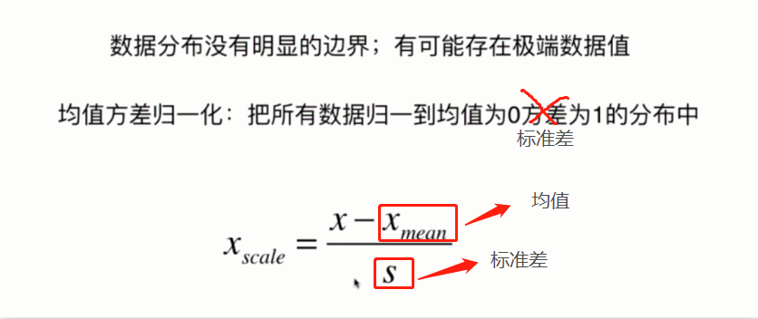
零均值标准化
或者叫均值标准差归一化
把所有数据都映射到均值为0标准差为1的分布中,这种归一化的方式则可以解决边界问题的。即便是没有明显边界,比如学生的成绩等等,也是可以使用这种方法的。
import numpy as np
x = np.random.randint(0, 100, size=(50, 2))
print(x)
"""
[[81 23]
 [38 58]
 [60 61]
 [ 1 98]
 [33 19]
 [10 43]
 [59  2]
 [93 33]
 [16 82]
 [10 94]
 [97 66]
 [25 76]
 [22 90]
 [64 88]
 [99 40]
 [90 80]
 [ 7 47]
 [41 28]
 [16 71]
 [ 3 51]
 [41 50]
 [32  9]
 [27 67]
 [ 3 37]
 [33 59]
 [42 77]
 [36 34]
 [52 29]
 [42  6]
 [30 60]
 [ 8 14]
 [54 99]
 [71 11]
 [37  6]
 [51 48]
 [10 58]
 [68 75]
 [ 1 50]
 [30  4]
 [21 66]
 [ 2 78]
 [57 67]
 [44 95]
 [16 52]
 [ 6 10]
 [26 38]
 [59 47]
 [17 28]
 [27 91]
 [59 12]]
"""
x_mean = np.mean(x, axis=0)
x_std = np.std(x, axis=0)
x = (x - x_mean) / x_std
print(x)
"""
[[ 1.64476893 -0.97317015]
 [ 0.02486366  0.26361109]
 [ 0.8536524   0.36962091]
 [-1.36900831  1.67707536]
 [-0.16349741 -1.11451658]
 [-1.02995837 -0.26643802]
 [ 0.81598019 -1.71523889]
 [ 2.09683551 -0.61980408]
 [-0.80392508  1.11168965]
 [-1.02995837  1.53572893]
 [ 2.24752437  0.54630394]
 [-0.46487514  0.89967001]
 [-0.57789178  1.3943825 ]
 [ 1.00434126  1.32370929]
 [ 2.3228688  -0.37244784]
 [ 1.98381886  1.04101644]
 [-1.14297502 -0.12509159]
 [ 0.13788031 -0.79648712]
 [-0.80392508  0.72298697]
 [-1.29366388  0.01625484]
 [ 0.13788031 -0.01908177]
 [-0.20116963 -1.46788265]
 [-0.38953071  0.58164055]
 [-1.29366388 -0.47845766]
 [-0.16349741  0.29894769]
 [ 0.17555252  0.93500662]
 [-0.05048077 -0.58446748]
 [ 0.55227468 -0.76115051]
 [ 0.17555252 -1.57389247]
 [-0.27651406  0.3342843 ]
 [-1.1053028  -1.29119961]
 [ 0.62761911  1.71241196]
 [ 1.26804677 -1.39720943]
 [-0.01280855 -1.57389247]
 [ 0.51460246 -0.08975498]
 [-1.02995837  0.26361109]
 [ 1.15503013  0.8643334 ]
 [-1.36900831 -0.01908177]
 [-0.27651406 -1.64456568]
 [-0.615564    0.54630394]
 [-1.33133609  0.97034322]
 [ 0.74063576  0.58164055]
 [ 0.25089695  1.57106554]
 [-0.80392508  0.05159145]
 [-1.18064723 -1.43254604]
 [-0.42720292 -0.44312105]
 [ 0.81598019 -0.12509159]
 [-0.76625286 -0.79648712]
 [-0.38953071  1.42971911]
 [ 0.81598019 -1.36187283]]
"""
print(np.mean(x))  # -4.218847493575595e-17
print(np.std(x))  # 0.9999999999999997
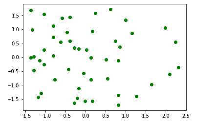
import matplotlib.pyplot as plt
%matplotlib inline
plt.scatter(x[:, 0], x[:, 1], color="g")
(八)sklearn中的Scaler
对测试数据集如何归一化
很容易想到,对训练数据集进行归一化,求出mean_train和std_train,归一化之后训练模型。然后再对测试数据集进行归一化求出mean_test和std_test,归一化之后进行预测不就可以可以了吗?
但是这样是不对的。
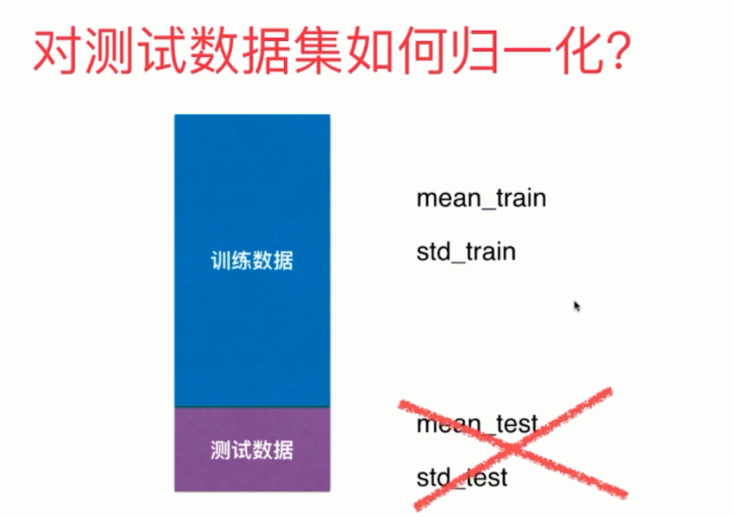
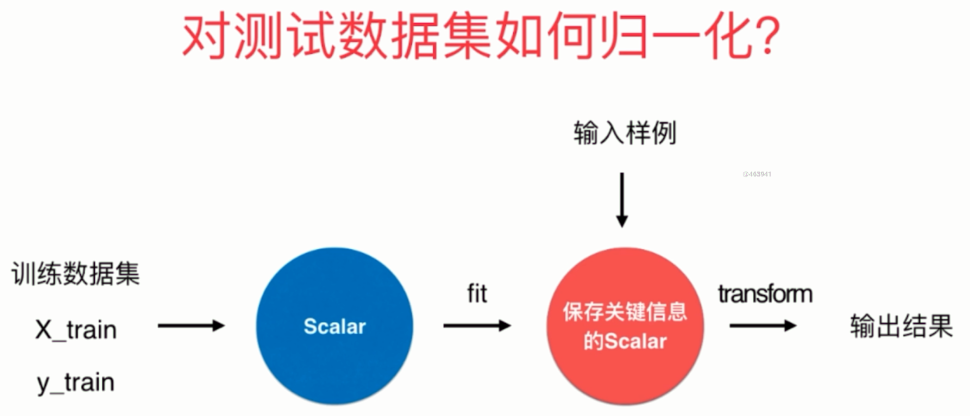
我们正确的做法是使用训练数据集的mean_train和std_train对测试数据集进行归一化。

原因如下:
测试数据是模拟真实环境
- 真实环境很有可能无法得到所有测试数据的均值与标准差
- 对数据的归一化也是算法的一部分
因此我们需要保存训练数据集得到的均值与标准差。这在sklearn中也提供了相应的算法,而且被封装成了一个类,并且这和其它算法的格式是类似的,在sklearn中,所有算法都保证了格式的统一。
from sklearn.datasets import load_iris
from sklearn.model_selection import train_test_split
from sklearn.preprocessing import StandardScaler
from sklearn.neighbors import KNeighborsClassifier


iris = load_iris()
X = iris.data
y = iris.target

X_train, X_test, y_train, y_test = train_test_split(X, y, test_size=0.3)

std_sca = StandardScaler()
# 这一步相当于计算出X_train中的mean和std
std_sca.fit(X_train)

# 查看均值和标准差
# 还记得这种结尾带下划线的参数吗?表示这种类型的参数不是我们传进去的,而是计算的时候生成的,还可以给我们后续使用的。
print(std_sca.mean_)  # [5.78285714 3.0552381  3.62190476 1.14285714]
print(std_sca.scale_)  # [0.78757701 0.45313321 1.73666242 0.74294871]

# 调用transform方法,对数据进行转化
scale_X_train = std_sca.transform(X_train)
scale_X_test = std_sca.transform(X_test)

knn_clf = KNeighborsClassifier()
# 对归一化之后的数据进行fit
knn_clf.fit(scale_X_train, y_train)
# 对归一化之后的数据进行打分
score = knn_clf.score(scale_X_test, y_test)
print(score)  # 1.0

# 由于鸢尾花数据集比较规整,当我们进行数据归一化的时候,分类准确率达到了百分之百
# 但是注意的是,当我们对训练数据集进行归一化处理的时候,对测试集也必须要进行归一化处理,如果不进行归一化处理的话,那么结果肯定是不准确的。
# 我们可以尝试使用原始的测试集进行预测,看看结果如何
print(knn_clf.score(X_test, y_test))  # 0.3333333333333333
# 可以看到结果的分数只有0.333,显而易见如果只对训练集进行归一化处理而不对测试数据集进行归一化处理的话,那么结果会非常糟糕
自己实现一个StandardScaler
其实sklearn还有很多其他的归一化方式,比如我们之前提到的最值归一化,这在sklearn中被封装为MinMaxScaler,有兴趣可以自己尝试,我们这里介绍零均值标准化
import numpy as np
from sklearn.datasets import load_iris
iris = load_iris()
X = iris.data


class MyStandardScaler:

    def __init__(self):
        # 这两个参数用户不需要传,而是根据训练自己生成
        self.mean_ = None
        self.scale_ = None

    def fit(self, X):
        # 根据训练集X得到均值和标准差
        self.mean_ = np.mean(X, axis=0)
        self.scale_ = np.std(X, axis=0)
        return self

    def transform(self, X):
        assert self.mean_ is not None, "在transform之前必须先fit"
        assert X.shape[1] == len(self.mean_)
        return (X - self.mean_) / self.scale_

    def __str__(self):
        return f"{self.__name__}(mean_: {self.mean_}, scale_: {self.scale_})"

    def __repr__(self):
        return f"{self.__name__}(mean_: {self.mean_}, scale_: {self.scale_})"


from sklearn.preprocessing import StandardScaler
std_sca = StandardScaler()

my_std_sca = MyStandardScaler()


std_sca.fit(X)
my_std_sca.fit(X)

print(std_sca.mean_, std_sca.scale_)
# [5.84333333 3.05733333 3.758      1.19933333] [0.82530129 0.43441097 1.75940407 0.75969263]

print(my_std_sca.mean_, my_std_sca.scale_)
# [5.84333333 3.05733333 3.758      1.19933333] [0.82530129 0.43441097 1.75940407 0.75969263]


print((std_sca.transform(X) == my_std_sca.transform(X)).all().all())  # True

# 可以看到我们自己实现的归一化和sklearn提供的归一化得到的是一样的结果。
(九)更多有关K近邻算法的思考
K近邻优点
K近邻算法用于解决分类问题,有些算法不适合解决分类问题,或者只适合解决二分类问题,而k近邻天然可以解决多分类问题。而且思想简单,功能强大
不仅如此,k近邻还可以解决回归问题。回归问题和分类问题不同,分类问题是预测出一个类别,换句话说,种类是有限个。而回归问题,则是预测出一个具体的数值,数字有千千万万个,肯定不能用分类来解决。
那既然如此的话,k近邻又如何解决回归问题呢?
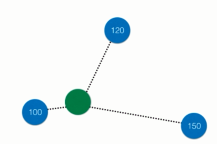
比如绿色的周围有三个点,那么k近邻可以取其平均值作为预测值,当然也可以考虑距离,采用加权平均的方式来计算。
事实上sklearn不仅提供了KNeighborsClassifier(k近邻分类),还提供了KNeighborsRegressor(k近邻回归),关于回归会在后面介绍。
K近邻缺点
- 最大的缺点:效率低下
如果训练集有m个样本,n个特征,则预测一个新的数据,时间复杂度是O(m*n),因为要和样本的每一个维度进行相减,然后平方相加、开方(按照欧拉距离),然后和m个样本重复相同的操作。
优化的话,可以使用树结构:KD-Tree,Ball-Tree,但即便如此,效率依旧不高
-
缺点二:高度数据相关
理论上,所有的数据都是高度相关的,但是k近邻对数据更加敏感。尤其是数据边界,哪怕只有一两个数据很远,也足以让我们的预测结果变得不准确,即使存在大量的正确样本
-
缺点三:预测结果不具有可解释性
k近邻得出的结果是不具备可解释的
-
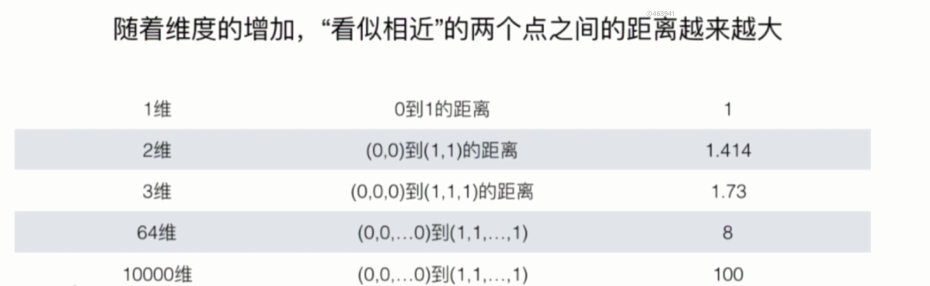
缺点四:维数灾难
随着维度的增加,看似相近的两个点之间的距离会越来越大
(十)机器学习流程回顾
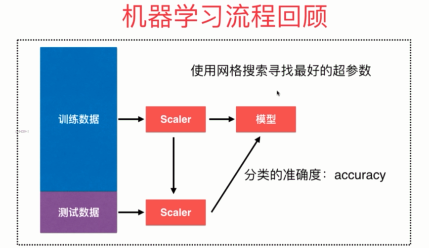
总结一下就是:
- 将数据集分成训练集合测试集
- 对训练集进行归一化,然后训练模型
- 对测试集使用同样的scaler(对测试训练的scaler)进行归一化,然后送到模型里面
- 网格搜索,通过分类准确度来寻找一个最好的超参数