pytorch基础

import torch
import time
a = torch.randn(10000, 1000)#要有空格
b = torch.randn(1000, 2000)#1000行，2000列的矩阵
t0 = time.time()
c = torch.matmul(a, b)#CPU模式的矩阵乘法
t1 = time.time()
print(a.device, t1-t0, c.norm(2))
cpu 0.534600019454956 tensor(140360.3125

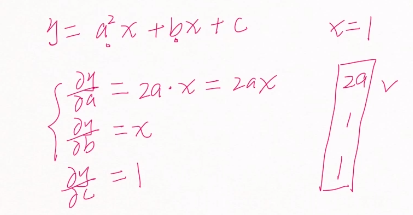
#自动求导数
import torch
import time
from torch import autograd
x = torch.tensor(1.)
a = torch.tensor(1., requires_grad=True)#a的初始值为1
b = torch.tensor(2., requires_grad=True)
c = torch.tensor(3., requires_grad=True)
y = a**2*x+b*x+c
print('before: ', a.grad, b.grad, c.grad)
grads = autograd.grad(y, [a, b, c])#求导
print('after: ', grads[0], grads[1], grads[2])

before:  None None None
after:  tensor(2.) tensor(1.) tensor(1.)

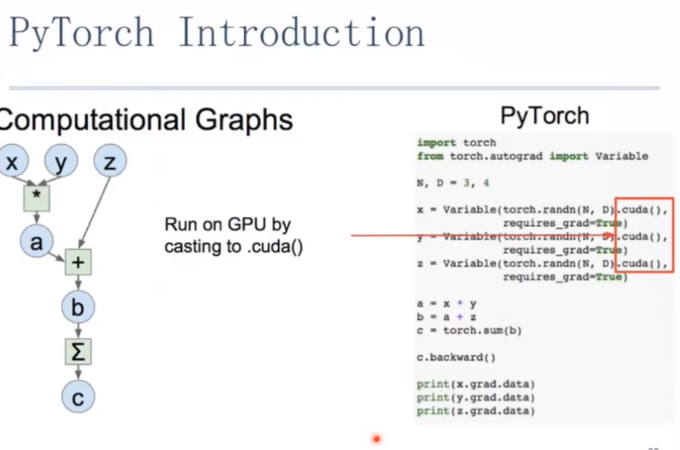
import torch
from torch.autograd import Variable
N,D = 3, 4
x = Variable(torch.randn(N,D),
             requires_grad = True)
#放在GPU上跑
x = Variable(torch.randn(N,D).cuda(),
             requires_grad = True)


y = Variable(torch.randn(N,D),
             requires_grad = True)
z = Variable(torch.randn(N,D),
             requires_grad = True)

a = x * y
b = a+z
c = torch.sum(b)

c.backward()#计算所有中间变量的导数

print(x.grad.data)
print(y.grad.data)
print(y.grad.data)

tensor([[-0.6182, 1.5300, -1.6665, -0.9114],
[ 0.2941, 0.3281, -0.0590, -2.4240],
[ 0.9295, -0.3222, -0.6462, 0.7567]])
tensor([[ 0.2332, 0.1874, 1.6639, 0.1480],
[ 0.9735, -1.0833, 1.4088, 0.2536],
[ 0.5914, 0.3669, -0.4866, -1.6782]])
tensor([[ 0.2332, 0.1874, 1.6639, 0.1480],
[ 0.9735, -1.0833, 1.4088, 0.2536],
[ 0.5914, 0.3669, -0.4866, -1.6782]])

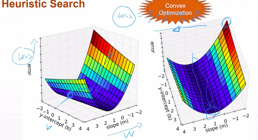
梯度下降 可以求极小值

 

核心;x = x -f'(x)×学习率(导数)#学习率为了更 精确的预测
在f'(x)=0处抖动，因为=0也会有误差 极小值

一般只要预测值是连续的，都叫回归问题
逻辑回归：用于预测属于某类的概率 (预测值在[0,1])，从这个角度理解，他就是2分类预测

 

 

 

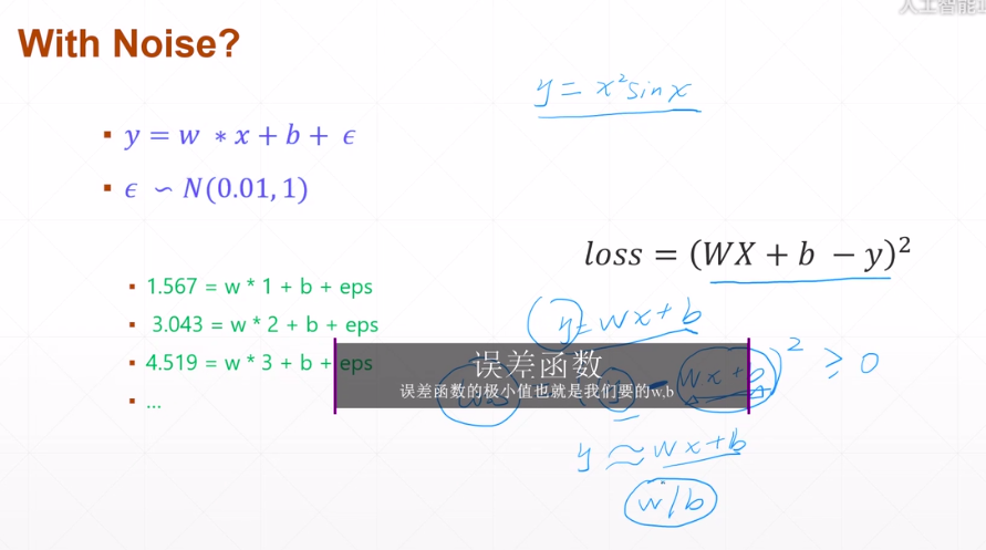
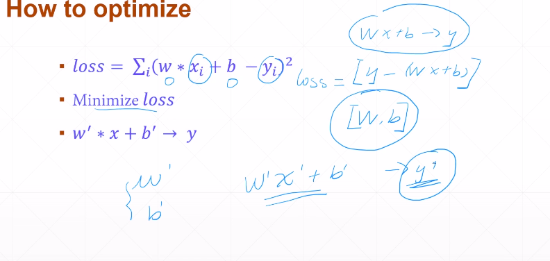
w,b在变动

 可参考这个博客https://blog.csdn.net/fanjianhai/article/details/103165530

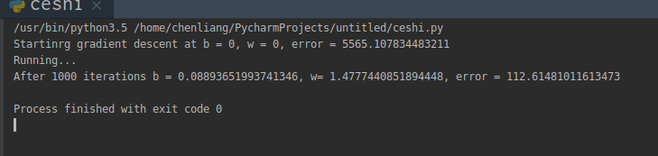
import numpy as np
# y = wx + b
def compute_error_for_point(b, w, points):
    total_error = 0
    for i in range(0, len(points)):
        x = points[i, 0]
        y = points[i, 1]
        total_error += (y - (w * x + b)) ** 2
    return total_error / float(len(points))

def step_grad(b_current, w_current, points, learn_rate):
    b_grad = 0
    w_grad = 0
    N = float(len(points))
    for i in range(0, len(points)):
        x = points[i, 0]
        y = points[i, 1]
       # grad_b = 2(wx+b-y)
        b_grad += -(2/N) * (y - ((w_current * x) + b_current))
        w_grad += -(2/N) * x * (y - ((w_current * x) + b_current))
        # grad_w = 2(wx+b-y)*x 求导数
    new_b = b_current - (learn_rate * b_grad)
    new_w = w_current - (learn_rate * w_grad)
    return [new_b, new_w]

def gradient_descent(points, start_b, start_w, learn_rate, num_iterator):
    b = start_b
    w = start_w
    for i in range(num_iterator):
        b, w = step_grad(b, w, np.array(points), learn_rate)
    return [b, w]

def run():
    points = np.genfromtxt("data.csv", delimiter=",")
    learn_rate = 0.0001
    init_b = 0 # initial y-intercept guess
    init_w = 0 # initial slope guess
    num_iterator =1000
    print("Startinrg gradient descent at b = {0}, w = {1}, error = {2}"
          .format(init_b, init_w,
                  compute_error_for_point(init_b, init_w, points))
          )
    print("Running...")
    [b, w] = gradient_descent(points, init_b, init_w, learn_rate, num_iterator)
    print("After {0} iterations b = {1}, w= {2}, error = {3}".
          format(num_iterator, b, w,
                 compute_error_for_point(b, w, points))
          )

if __name__ == '__main__':#name 前后都是__
    run()

 

 

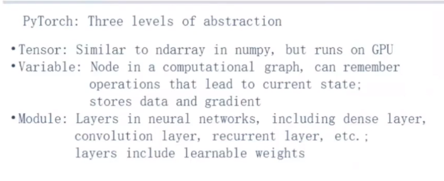
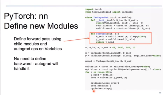
forawrd :给我一个值，输出是什么
backward:算出所给值的梯度

 model就像一个黑箱子

 

pytorch  和 tensorflow的区别

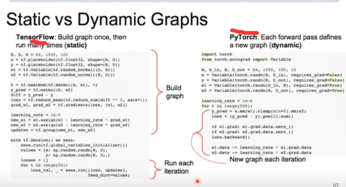
 static vs  dynamic

 

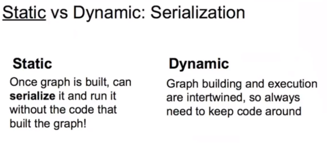
S 图建好后就不会再变了，只是运行不同的数据
D 网络的结构依赖数据

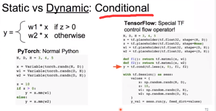
下面举个例子

条件语句

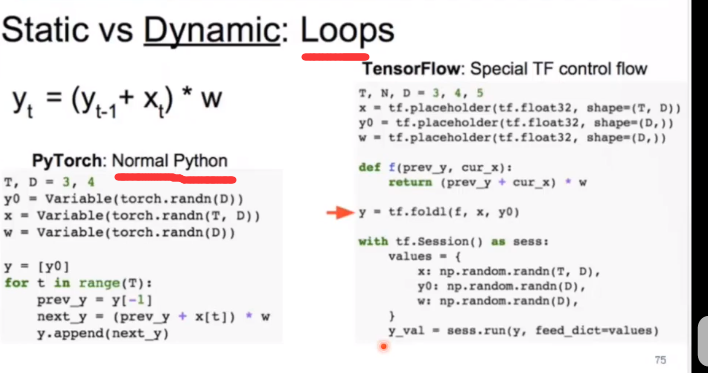
 循环语句

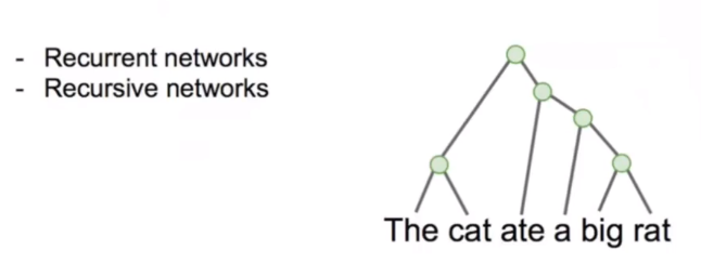
动态图应用

 

# a = [1,2,3,4]
# b =2
# b = torch.tensor(b)
# print(b)
# print(a[-b])
# print(a[-1])
tensor(2)
3
4

index = [1,2]
a = torch.randn(2,4,3,3)
print(a)
b = a[:,index,:,:]
print("b...:")
print(b)
print("b[0] : ")
print(b[0,:,:,:])
print(b.shape)


tensor([[[[ 0.2459,  0.6848,  0.6760],
          [-0.4188,  1.0681, -0.2383],
          [-0.9828, -1.1747,  0.3324]],

         [[ 0.6581, -0.9526,  0.7707],
          [-2.2539,  0.4771, -0.3570],
          [ 0.6010, -1.3780, -0.6772]],

         [[ 0.3594,  1.2516, -0.2323],
          [-0.2046,  0.8003,  0.6854],
          [-0.6111,  0.6822,  0.7537]],

         [[-1.3420, -0.6598,  0.6166],
          [ 0.8173,  1.1564,  0.1675],
          [-1.4180,  1.2084,  0.3865]]],


        [[[-0.7158,  0.1544, -0.2652],
          [-0.4343, -1.0831,  2.3954],
          [-0.0833,  0.0873,  0.0119]],

         [[ 0.4938, -0.2763,  0.3849],
          [ 1.7344,  0.3378,  0.0441],
          [-1.5186, -0.3244,  0.6782]],

         [[-0.3352,  1.4274, -0.3388],
          [ 1.2715,  0.0174,  2.0127],
          [ 0.4551,  0.5362, -0.1565]],

         [[ 0.1222,  0.0120, -0.8316],
          [ 0.2476,  1.4280,  0.3954],
          [-0.6422, -0.7224, -0.5245]]]])
b...:
tensor([[[[ 0.6581, -0.9526,  0.7707],
          [-2.2539,  0.4771, -0.3570],
          [ 0.6010, -1.3780, -0.6772]],

         [[ 0.3594,  1.2516, -0.2323],
          [-0.2046,  0.8003,  0.6854],
          [-0.6111,  0.6822,  0.7537]]],


        [[[ 0.4938, -0.2763,  0.3849],
          [ 1.7344,  0.3378,  0.0441],
          [-1.5186, -0.3244,  0.6782]],

         [[-0.3352,  1.4274, -0.3388],
          [ 1.2715,  0.0174,  2.0127],
          [ 0.4551,  0.5362, -0.1565]]]])
b[0] :
tensor([[[ 0.6581, -0.9526,  0.7707],
         [-2.2539,  0.4771, -0.3570],
         [ 0.6010, -1.3780, -0.6772]],

        [[ 0.3594,  1.2516, -0.2323],
         [-0.2046,  0.8003,  0.6854],
         [-0.6111,  0.6822,  0.7537]]])
torch.Size([2, 2, 3, 3])