原文链接:http://tecdat.cn/?p=9448
NASA有32,000多个数据集,并且NASA有兴趣了解这些数据集之间的联系,以及与NASA以外其他政府组织中其他重要数据集的联系。有关NASA数据集的元数据 可以JSON格式在线获得。让我们使用tf-idf在描述字段中找到重要的单词,并将其与关键字联系起来。
获取和整理NASA元数据
让我们下载32,000多个NASA数据集的元数据。
library(jsonlite)
library(dplyr)
library(tidyr)
metadata <- fromJSON("data.json")
names(metadata$dataset)
##  [1] "_id"                "@type"              "accessLevel"        "accrualPeriodicity"
##  [5] "bureauCode"         "contactPoint"       "description"        "distribution"
##  [9] "identifier"         "issued"             "keyword"            "landingPage"
## [13] "language"           "modified"           "programCode"        "publisher"
## [17] "spatial"            "temporal"           "theme"              "title"
## [21] "license"            "isPartOf"           "references"         "rights"
## [25] "describedBy"
nasadesc <- data_frame(id = metadata$dataset$`_id`$`$oid`, desc = metadata$dataset$description)
nasadesc
## # A tibble: 32,089 x 2
##                          id
##                       <chr>
## 1  55942a57c63a7fe59b495a77
## 2  55942a57c63a7fe59b495a78
## 3  55942a58c63a7fe59b495a79
## 4  55942a58c63a7fe59b495a7a
## 5  55942a58c63a7fe59b495a7b
## 6  55942a58c63a7fe59b495a7c
## 7  55942a58c63a7fe59b495a7d
## 8  55942a58c63a7fe59b495a7e
## 9  55942a58c63a7fe59b495a7f
## 10 55942a58c63a7fe59b495a80
## # ... with 32,079 more rows, and 1 more variables: desc <chr>
## # A tibble: 32,089 x 2
## id
## <chr>
## 1 55942a57c63a7fe59b495a77
## 2 55942a57c63a7fe59b495a78
## 3 55942a58c63a7fe59b495a79
## 4 55942a58c63a7fe59b495a7a
## 5 55942a58c63a7fe59b495a7b
## 6 55942a58c63a7fe59b495a7c
## 7 55942a58c63a7fe59b495a7d
## 8 55942a58c63a7fe59b495a7e
## 9 55942a58c63a7fe59b495a7f
## 10 55942a58c63a7fe59b495a80
## # ... with 32,079 more rows, and 1 more variables: desc <chr>让我们打印出其中的一部分。
nasadesc %>% select(desc) %>% sample_n(5)
## # A tibble: 5 x 1
##                                                                                                                                                      desc
##                                                                                                                                                     <chr>
## 1  A Group for High Resolution Sea Surface Temperature (GHRSST) Level 4 sea surface temperature analysis produced as a retrospective dataset at the JPL P
## 2  ML2CO is the EOS Aura Microwave Limb Sounder (MLS) standard product for carbon monoxide derived from radiances measured by the 640 GHz radiometer. The
## 3                                                                                                              Crew lock bag. Polygons: 405 Vertices: 514
## 4  JEM Engineering proved the technical feasibility of the FlexScan array?a very low-cost, highly-efficient, wideband phased array antenna?in Phase I, an
## 5 MODIS (or Moderate Resolution Imaging Spectroradiometer) is a key instrument aboard the
Terra (EOS AM) and Aqua (EOS PM) satellites. Terra's orbit aro
这是关键词。
nasakeyword <- data_frame(id = metadata$dataset$`_id`$`$oid`,
                          keyword = metadata$dataset$keyword) %>%
        unnest(keyword)
nasakeyword
## # A tibble: 126,814 x 2
## id keyword
## <chr> <chr>
## 1 55942a57c63a7fe59b495a77 EARTH SCIENCE
## 2 55942a57c63a7fe59b495a77 HYDROSPHERE
## 3 55942a57c63a7fe59b495a77 SURFACE WATER
## 4 55942a57c63a7fe59b495a78 EARTH SCIENCE
## 5 55942a57c63a7fe59b495a78 HYDROSPHERE
## 6 55942a57c63a7fe59b495a78 SURFACE WATER
## 7 55942a58c63a7fe59b495a79 EARTH SCIENCE
## 8 55942a58c63a7fe59b495a79 HYDROSPHERE
## 9 55942a58c63a7fe59b495a79 SURFACE WATER
## 10 55942a58c63a7fe59b495a7a EARTH SCIENCE
## # ... with 126,804 more rows最常见的关键字是什么?
nasakeyword %>% group_by(keyword) %>% count(sort = TRUE)
## # A tibble: 1,774 x 2
##                    keyword     n
##                      <chr> <int>
## 1            EARTH SCIENCE 14362
## 2                  Project  7452
## 3               ATMOSPHERE  7321
## 4              Ocean Color  7268
## 5             Ocean Optics  7268
## 6                   Oceans  7268
## 7                completed  6452
## 8  ATMOSPHERIC WATER VAPOR  3142
## 9                   OCEANS  2765
## 10            LAND SURFACE  2720
## # ... with 1,764 more rows
看起来“已完成项目”对于某些目的来说可能不是有用的关键字,我们可能希望将所有这些都更改为小写或大写,以消除诸如“ OCEANS”和“ Oceans”之类的重复项。
nasakeyword <- nasakeyword %>% mutate(keyword = toupper(keyword))
计算文字的tf-idf
什么是tf-idf?评估文档中单词的重要性的一种方法可能是其 术语频率 (tf),即单词在文档中出现的频率。但是,一些经常出现的单词并不重要。在英语中,这些词可能是“ the”,“ is”,“ of”等词。另一种方法是查看术语的 逆文档频率 (idf),这会降低常用单词的权重,而增加在文档集中很少使用的单词的权重。
library(tidytext)
descwords <- nasadesc %>% unnest_tokens(word, desc) %>%
        count(id, word, sort = TRUE) %>%
        ungroup()
descwords
## # A tibble: 2,728,224 x 3
## id word n
## <chr> <chr> <int>
## 1 55942a88c63a7fe59b498280 amp 679
## 2 55942a88c63a7fe59b498280 nbsp 655
## 3 55942a8ec63a7fe59b4986ef gt 330
## 4 55942a8ec63a7fe59b4986ef lt 330
## 5 55942a8ec63a7fe59b4986ef p 327
## 6 55942a8ec63a7fe59b4986ef the 231
## 7 55942a86c63a7fe59b49803b amp 208
## 8 55942a86c63a7fe59b49803b nbsp 204
## 9 56cf5b00a759fdadc44e564a the 201
## 10 55942a86c63a7fe59b4980a2 gt 191
## # ... with 2,728,214 more rows这些是NASA说明字段中最常见的“单词”,是词频最高的单词。让我们看一下第一个数据集,例如:
nasadesc %>% filter(id == "55942a88c63a7fe59b498280") %>% select(desc)
## # A tibble: 1 x 1
## desc
## <chr>
## 1 <p>The objective of the Variable Oxygen Regulator Element is to develop an oxygen-rated, contaminant-tolerant oxygen regulator to control suit ptf-idf算法应该减少所有这些的权重,因为它们很常见,但是我们可以根据需要通过停用词将其删除。现在,让我们为描述字段中的所有单词计算tf-idf。
descwords <- descwords %>% bind_tf_idf(word, id, n)
descwords
## # A tibble: 2,728,224 x 6
## id word n tf idf tf_idf
## <chr> <chr> <int> <dbl> <dbl> <dbl>
## 1 55942a88c63a7fe59b498280 amp 679 0.35661765 3.1810813 1.134429711
## 2 55942a88c63a7fe59b498280 nbsp 655 0.34401261 4.2066578 1.447143322
## 3 55942a8ec63a7fe59b4986ef gt 330 0.05722213 3.2263517 0.184618705
## 4 55942a8ec63a7fe59b4986ef lt 330 0.05722213 3.2903671 0.188281801
## 5 55942a8ec63a7fe59b4986ef p 327 0.05670192 3.3741126 0.191318680
## 6 55942a8ec63a7fe59b4986ef the 231 0.04005549 0.1485621 0.005950728
## 7 55942a86c63a7fe59b49803b amp 208 0.32911392 3.1810813 1.046938133
## 8 55942a86c63a7fe59b49803b nbsp 204 0.32278481 4.2066578 1.357845252
## 9 56cf5b00a759fdadc44e564a the 201 0.06962245 0.1485621 0.010343258
## 10 55942a86c63a7fe59b4980a2 gt 191 0.12290862 3.2263517 0.396546449
## # ... with 2,728,214 more rows添加的列是tf,idf,这两个数量相乘在一起是tf-idf,这是我们感兴趣的东西。NASA描述字段中最高的tf-idf词是什么?
descwords %>% arrange(-tf_idf)
## # A tibble: 2,728,224 x 6
##                          id                                          word     n    tf       idf
##                       <chr>                                         <chr> <int> <dbl>     <dbl>
## 1  55942a7cc63a7fe59b49774a                                           rdr     1     1 10.376269
## 2  55942ac9c63a7fe59b49b688 palsar_radiometric_terrain_corrected_high_res     1     1 10.376269
## 3  55942ac9c63a7fe59b49b689  palsar_radiometric_terrain_corrected_low_res     1     1 10.376269
## 4  55942a7bc63a7fe59b4976ca                                          lgrs     1     1  8.766831
## 5  55942a7bc63a7fe59b4976d2                                          lgrs     1     1  8.766831
## 6  55942a7bc63a7fe59b4976e3                                          lgrs     1     1  8.766831
## 7  55942ad8c63a7fe59b49cf6c                      template_proddescription     1     1  8.296827
## 8  55942ad8c63a7fe59b49cf6d                      template_proddescription     1     1  8.296827
## 9  55942ad8c63a7fe59b49cf6e                      template_proddescription     1     1  8.296827
## 10 55942ad8c63a7fe59b49cf6f                      template_proddescription     1     1  8.296827
##       tf_idf
##        <dbl>
## 1  10.376269
## 2  10.376269
## 3  10.376269
## 4   8.766831
## 5   8.766831
## 6   8.766831
## 7   8.296827
## 8   8.296827
## 9   8.296827
## 10  8.296827
## # ... with 2,728,214 more rows
因此,这些是用tf-idf衡量的描述字段中最“重要”的词,这意味着它们很常见,但不太常用。
nasadesc %>% filter(id == "55942a7cc63a7fe59b49774a") %>% select(desc)
## # A tibble: 1 x 1
##    desc
##   <chr>
## 1   RDR
tf-idf算法将认为这是一个非常重要的词。
连接关键字和描述
因此,现在我们知道描述中的哪个词具有较高的tf-idf,并且在关键字中也有这些描述的标签。
descwords <- full_join(descwords, nasakeyword, by = "id")
descwords
## # A tibble: 11,013,838 x 7
## id word n tf idf tf_idf keyword
## <chr> <chr> <int> <dbl> <dbl> <dbl> <chr>
## 1 55942a88c63a7fe59b498280 amp 679 0.35661765 3.181081 1.1344297 ELEMENT
## 2 55942a88c63a7fe59b498280 amp 679 0.35661765 3.181081 1.1344297 JOHNSON SPACE CENTER
## 3 55942a88c63a7fe59b498280 amp 679 0.35661765 3.181081 1.1344297 VOR
## 4 55942a88c63a7fe59b498280 amp 679 0.35661765 3.181081 1.1344297 ACTIVE
## 5 55942a88c63a7fe59b498280 nbsp 655 0.34401261 4.206658 1.4471433 ELEMENT
## 6 55942a88c63a7fe59b498280 nbsp 655 0.34401261 4.206658 1.4471433 JOHNSON SPACE CENTER
## 7 55942a88c63a7fe59b498280 nbsp 655 0.34401261 4.206658 1.4471433 VOR
## 8 55942a88c63a7fe59b498280 nbsp 655 0.34401261 4.206658 1.4471433 ACTIVE
## 9 55942a8ec63a7fe59b4986ef gt 330 0.05722213 3.226352 0.1846187 JOHNSON SPACE CENTER
## 10 55942a8ec63a7fe59b4986ef gt 330 0.05722213 3.226352 0.1846187 PROJECT
## # ... with 11,013,828 more rows可视化结果
让我们来看几个示例关键字中最重要的单词。
plot_words <- descwords %>% filter(!near(tf, 1)) %>%
        filter(keyword %in% c("SOLAR ACTIVITY", "CLOUDS",
                              "VEGETATION", "ASTROPHYSICS",
                              "HUMAN HEALTH", "BUDGET")) %>%
        arrange(desc(tf_idf)) %>%
        group_by(keyword) %>%
        distinct(word, keyword, .keep_all = TRUE) %>%
        top_n(20, tf_idf) %>% ungroup() %>%
        mutate(word = factor(word, levels = rev(unique(word))))
plot_words
## # A tibble: 122 x 7
## id word n tf idf tf_idf keyword
## <chr> <fctr> <int> <dbl> <dbl> <dbl> <chr>
## 1 55942a60c63a7fe59b49612f estimates 1 0.5000000 3.172863 1.586432 CLOUDS
## 2 55942a76c63a7fe59b49728d ncdc 1 0.1666667 7.603680 1.267280 CLOUDS
## 3 55942a60c63a7fe59b49612f cloud 1 0.5000000 2.464212 1.232106 CLOUDS
## 4 55942a5ac63a7fe59b495bd8 fife 1 0.2000000 5.910360 1.182072 CLOUDS
## 5 55942a5cc63a7fe59b495deb allometry 1 0.1428571 7.891362 1.127337 VEGETATION
## 6 55942a5dc63a7fe59b495ede tgb 3 0.1875000 5.945452 1.114772 VEGETATION
## 7 55942a5ac63a7fe59b495bd8 tovs 1 0.2000000 5.524238 1.104848 CLOUDS
## 8 55942a5ac63a7fe59b495bd8 received 1 0.2000000 5.332843 1.066569 CLOUDS
## 9 55942a5cc63a7fe59b495dfd sap 1 0.1250000 8.430358 1.053795 VEGETATION
## 10 55942a60c63a7fe59b496131 abstract 1 0.3333333 3.118561 1.039520 CLOUDS
## # ... with 112 more rowsnasadesc %>% filter(id == "55942a60c63a7fe59b49612f") %>% select(desc)
## # A tibble: 1 x 1
##              desc
##             <chr>
## 1 Cloud estimates
tf-idf算法在仅2个字长的描述中无法很好地工作,或者至少它将对这些字进行非常重的加权。实际上,也许这是不合适的。
library(ggplot2)
library(ggstance)
library(ggthemes)
ggplot(plot_words, aes(tf_idf, word, fill = keyword, alpha = tf_idf)) +
        geom_barh(stat = "identity", show.legend = FALSE) +
        labs(title = "Highest tf-idf words in NASA Metadata Description Fields",
             subtitle = "Distribution of tf-idf for words from datasets labeled with various keywords",
             caption = "NASA metadata from https://data.nasa.gov/data.json",
             y = NULL, x = "tf-idf") +
        facet_wrap(~keyword, ncol = 3, scales = "free") +
        theme_tufte(base_family = "Arial", base_size = 13, ticks = FALSE) +
        scale_alpha_continuous(range = c(0.2, 1)) +
        scale_x_continuous(expand=c(0,0)) +
        theme(strip.text=element_text(hjust=0)) +
        theme(plot.caption=element_text(size=9))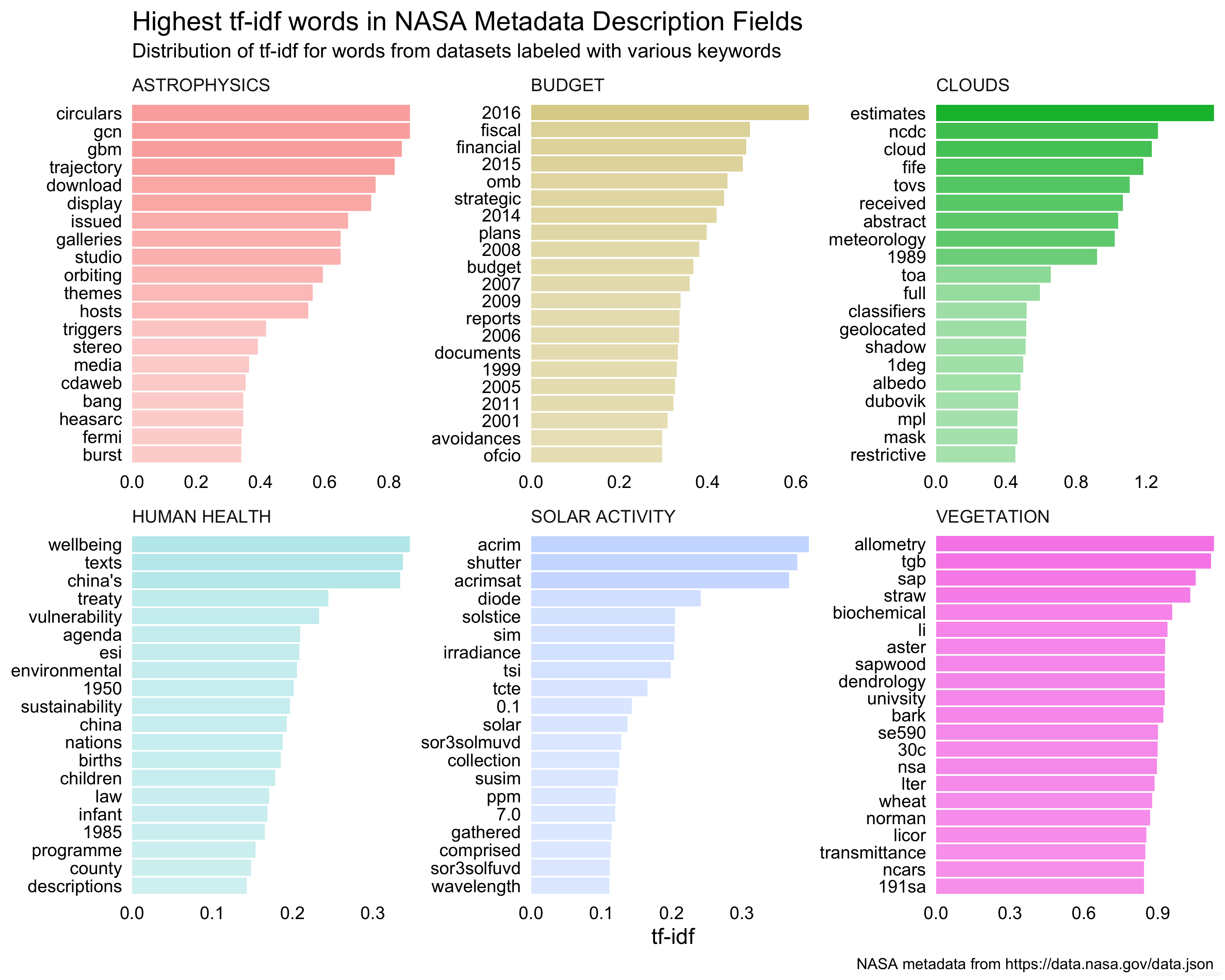
![]()