This link proides a variety of completements of all kinds fo image processing methods.
https://www.peterkovesi.com/
https://www.peterkovesi.com/matlabfns/index.html

MATLAB and Octave Functions
for Computer Vision and Image Processing
Peter Kovesi |
Index to Code Sections
The complete set of these functions is available as a zip fileMatlabFns.zip
MATLABTo use these functions you will need MATLAB and the MATLAB Image Processing Toolbox. |
OctaveAlternatively you can use Octave which is a very good open source alternative to MATLAB. Almost all the functions on this page run under Octave. See my Notes on using Octave. An advantage of using Octave is that you can run it on your Android device. (I can compute phase congruency on my mobile phone!) Get Corbin Champion's port of Octave at Google play here. MATLAB/Octave compatibility of individual function is indicated as follows
|
Perceptually Uniform Colour Maps
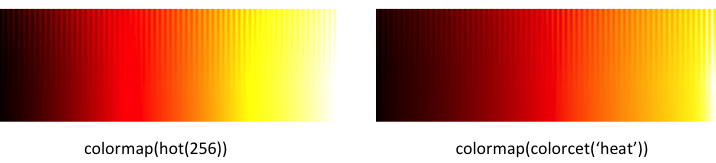
Many widely used colour maps have perceptual flat spots that can hide features as large as 10% of your total data range. They may also have points of locally high colour contrast leading to the perception of false features in your data when there are none. MATLAB's 'hot', 'jet', and 'hsv' colour maps suffer from these problems. Use the perceptually uniform colorcet maps instead! For an overview of this work and the theory behind it please visit this page.
- colorcet.m A stand-alone function that contains pre-generated arrays of my perceptually uniform colour maps.
If you are to download just one function from this page get this one!
Generation and correction of colour maps
If you want to experiment with the generation of your own perceptually uniform colour maps...
- cmap.m Colour map generating function. Select from a large library of colour maps. Colour maps are defined by B-spline paths through CIELAB space. The parameterisation along the path is then adjusted to ensure uniform perceptual contrast. Modify the function to add any new colour maps you want.
- equalisecolourmap.m Remaps entries in a colour map in order to equalise the perceptual contrast across the colour map. Used by cmap.m . Can also be used to 'rescue' some of MATLAB's colour maps.
- linearrgbmap.m Generates a linear colour map from [0 0 0] to a specified colour in RGB space.
- ternarymaps.m Returns three basis/primary colour maps for generating ternary images. The colour maps are closely matched in lightness (unlike the RGB primaries).
- randmap.m Generates a colour map of random colours. Not perceptually uniform and certainly not useful for displaying data that varies over a continous range. However, it is useful for displaying a labeled segmented image.
- makecolorcet.m Used to automatically generate the colorcet.m function using cmap.m
- pseudogrey.m Pseudogrey scale colour map with 2551 levels. This colour map may help if you are wanting to get the best possible rendering of a high dynamic range greyscale image on an 8 bit display.
Rendering of images with colour maps
- applycolourmap.m Applies a colour map to a single channel image to obtain an RGB result.
- showdivim.m This function is intended for displaying an image with a diverging colour map. To do this correctly requires that the desired reference value in the data is correctly associated with the centre entry of the diverging colour map.
- showangularim.m This function displays an image of angular data with a specified colour map. For angular data to be rendered correctly it is important that the data values are respected so that data values are correctly assigned to specific entries in a cyclic colour map. The assignment of values to colours also depends on whether the data is cyclic over pi, or 2*pi. This function also allows the colour map encoding of the angular information to be modulated to represent the amplitude/reliability/coherence of the angular data.
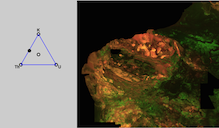
Ternary Images
- ternaryimage.m Generates a perceptually uniform ternary image from 3 bands of data.
Requires
Test images
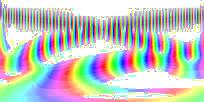
- sineramp.m Generates a test image consisting of a sine wave superimposed on a ramp function The amplitude of the sine wave is modulated from its full value at the top of the image to 0 at the bottom. A useful test image for evaluating colour maps.
- circlesineramp.m Generates a test image representing a cyclic version of sineramp.m for testing of cyclic colour maps. It consists of a sine wave superimposed on a spiral ramp function.
Visualization of colour map paths and colour spaces
- colourmappath.m Plots the path of a colour map through CIELAB or RGB colour spaces.
- viewlabspace.m Interactive visualization of CIELAB colour space. Useful for charting locations of spline control points for defining colour maps with cmap.m
- viewlabspace2.m Another interactive visualization of CIELAB colour space that provides vertical slices through the colour space.
- generatelabslice.m Generates an RGB image of a slice throught CIELAB space at a specified lightness level.
Functions for reading and writing colour maps in various formats
- writecolourmapfn.m Creates a MATLAB function file from a Nx3 colour map.
- map2geosofttbl.m Writes a RGB colour map to a .tbl file for use with Geosoft Oasis Montaj or QGIS.
- map2ermapperlutfile.m Writes a colour map to a .lut file for use with ER Mapper, Intrepid or MapInfo.
- readermapperlutfile.m Reads a colour map in ER Mapper's LUT format.
- map2imagejlutfile.m Writes a colour map to a .lut file for use with ImageJ.
- readimagejlutfile.m Reads a colour map in ImageJ's LUT format.
- map2actfile.m Writes a colour map to an Adobe Colour Map Table .act file.
- map2qgisstyle.m Writes colour maps to a QGIS xml style file.
Colour blindness simulation and visualization.
- colourblind.m Simulates colour appearance for colour blind viewers.
- colourblindlabspace.m Visualization of colour blind colour spaces in Lab space. Used to support the design of colour maps for the colour blind.
- colourblindlmsspace.m Visualization of colour blind colour spaces in LMS space.
Colour space conversions.
- rgb2lab.m RGB to L*a*b* colour conversion.
- rgb2cmyk.m RGB to cmyk colour conversion.
- cmyk2rgb.m cmyk to RGB colour conversion.
- rgb2lms.m RGB colours to LMS cone responses.
- lms2rgb.m LMS cone responses to RGB colours.
- xyz2lms.m XYZ to LMS cone responses.
- rgb2nrgb.m RGB to normalized RGB colour conversion.
Additional supporting functions that are required.
- bbspline.m Basic b-spline implementation used to generate paths through colour space for cmap.m
- pbspline.m Basic periodic b-spline implementation used to generate paths through colour space for cmap.m
- Also needed: show.m, normalise.m and strendswith.m
Julia Code
- For those working in Julia I have produced a package containing most of the functions above: PerceptualColourMaps.jl
Python Colour Maps
- For those working in Python these colour maps are available at github.com/bokeh/colorcet. This package gives you access to these colour maps for use with Python plotting programs such as Bokeh, Matplotlib, HoloViews, GeoViews, and Datashader. Thanks to James Bednar.
R Colour Maps
- For those working in R these colour maps are available in the cetcolor package maintained by James Balamuta. They are also incorporated in thepals package maintained by Kevin Wright. The pals package gathers together a number of colour maps including the CET perceptually uniform colour maps and also includes R code for generating the colour map test image.
Reference:
- Peter Kovesi. "Good Colour Maps: How to Design Them."
arXiv:1509.03700 [cs.GR] 2015.
Interactive Image Blending
These functions provide a set of interactive tools for visualizing multiple images. Some videos of their use can be seen here.
- linimix.m Generates an interactive image for blending between a sequence of images.
- bilinimix.m Generates an interactive image for blending between a 2D grid of images.
- ternarymix.m Interactive ternary image for blending 3 images. You can also switch between blending and swiping modes.
Updated December 2014 to incorporate swiping in addition to blending. Can also switch between colour and greyscale modes. - binarymix.m Just like ternarymix but for 2 images.
- cliquemix.m Allows blending or swiping between any pair within a collection of images.
Updated December 2014 to incorporate swiping in addition to blending. - cyclemix.m Allows blending between a sequence of images in a cyclic manner.
- logisticweighting.m Adaptation of the generalised logistics function for use as a weighting function for blending images.
- swipe.m Don't just swipe between two images when you can interactively swipe between 2, 3 or 4 images!
- collectncheckimages.m Collects and checks images prior to blending.
The functions above also require: normalise.m, histtruncate.m, circle.m, circularstruct.m and namenpath.m.
Demo package: Download BlendDemo.zip. This contains all the functions above and some sample data sets. Within the expanded folder in MATLAB run blenddemo.m. A series of windows will open, each demonstrating a different blending interface. Click in any of them and play!
Reference:
- Peter Kovesi, Eun-Jung Holden and Jason Wong, 2014. "Interactive Multi-Image Blending for Visualization and Interpretation," Computers & Geosciences 72 (2014) 147-155. http://doi.org/10.1016/j.cageo.2014.07.010
Phase Based Feature Detection and Phase Congruency
Phase congruency is an illumination and contrast invariant measure of feature significance. Unlike gradient based feature detectors, which can only detect step features, phase congruency correctly detects features at all kind of phase angle, and not just step features having a phase angle of 0 or 180 degrees.
- phasecongmono.m This function computes phase congruency via monogenic filters. It has excellent speed and much reduced memory requirements compared to the other phase congruency functions below. Requires perfft2.m, filtergrid.m and lowpassfilter.m
- phasecong3.m This function supersedes phasecong2.m and phasecong.m being faster and requiring less memory. Computes corner features in addition to edges. Requires filtergrid.m and lowpassfilter.m
- Deprecated: phasecong.m Original code for calculating phase congruency in an image. This function also returns a feature type image. Note this function is superseded by phasecong2.m and phasecong3.m and is only here for reference.
- Deprecated: phasecong2.m Phase congruency code that combines edge and corner detection, and provides better localization. Note this function is superseded by phasecong3.m and phasecongmono.m and is only here for reference.
- dispfeat.m This function provides visualisation and statistics of the different feature types found in an image by phasecong. Typically you will find a broad distribution of all feature types between step edges and lines. This function needs edgelink.m (see below).
- odot.m Demonstrates the actions of the 'Odot' and 'Oslash' operators on a 1D signal. These operators allow one to decompose and combine signals in a way that is consistent with the Local Energy model of feature perception.
- spatialgabor.m applies a single oriented Gabor filter to an image.
phase symmetry image - phasesym.m Code for calculating phase symmetry. This can be used as a line and blob detector. Phase symmetry is an illumination and contrast invariant measure of symmetry in an image. (A bright circle is not more 'symmetric' than a grey circle as can be the case with some other measures!).
- phasesymmono.m This function computes phase symmetry via monogenic filters. Has excellent speed and much reduced memory requirements compared to phasesym.m However you may prefer the output from phasesym's oriented filters.
- gaborconvolve.m Code for convolving an image with a bank of log-Gabor filters. A pre-processing step for texture analysis, feature detection and classification, etc.
- plotgaborfilters.m A function for plotting log-Gabor filters. This function is useful for seeing what effect the various parameter settings have on the formation of a log-Gabor filter bank used in the functions above.
- monofilt.m An implementation of Felsberg's monogenic filters. This function applies a bank of monogenic filters to an image to obtain the 2D analytic signal over a number of scales. As in gaborconvolve this can be used as a pre-processing step for texture analysis, feature detection and classification, etc.
- highpassmonogenic.m Applies highpassfilter and computes phase and amplitude via monogenic filters. Requires perfft2.m
- filtergrid.m Generates grid for constructing frequency domain filters. Used by some of the functions above.
- An explanation of the implementation of convolution with log-Gabor filters used in the functions above.
References:
- Peter Kovesi, "Symmetry and Asymmetry From Local Phase". AI'97, Tenth Australian Joint Conference on Artificial Intelligence. 2 - 4 December 1997. Proceedings - Poster Papers. pp 185-190.
- Peter Kovesi, "Image Features From Phase Congruency". Videre: A Journal of Computer Vision Research. MIT Press. Volume 1, Number 3, Summer 1999.
Electronic publishing, even with a reputable publisher, can be problematic. For some reason the MIT Press has chosen to no longer maintain an archive of Videre. Fortunately an archive of the journal can be found at the University of Rochester at www.cs.rochester.edu/u/brown/Videre. - Peter Kovesi, "Edges Are Not Just Steps". Proceedings of ACCV2002 The Fifth Asian Conference on Computer Vision, Melbourne Jan 22-25, 2002. pp 822-827. (preprint)
- Peter Kovesi, "Phase Congruency Detects Corners and Edges". The Australian Pattern Recognition Society Conference: Digital Image Computing: Techniques and Applications DICTA 2003. December 2003. Sydney. pp 309-318. (preprint)
- Peter Kovesi, "Invariant Measures of Image Features From Phase Information". PhD Thesis, The University of Western Australia. 1996. Download page
 For those working in Julia the package ImagePhaseCongruency.jl implements most of the functions above.
Spatial Feature Detection
- canny.m Canny edge detector.
- harris.m Harris corner detector.
- noble.m Noble's corner detector.
- shi_tomasi.m The Shi-Tomasi corner detector returns the minimum eigenvalue of the structure tensor. This represents the ideal that the Harris and Noble detectors attempt to approximate.
- hessianfeatures.m Hessian feature detector.
- fastradial.m An implementation of Loy and Zelinski's fast radial feature detector.
- gaussfilt.m Wrapper function for convenient Gaussian filtering.
- derivative5.m computes 1st and 2nd derivatives of an image using the 5-tap coefficients given by Farid and Simoncelli. Use this function instead of MATLAB's GRADIENT function for much more accurate results.
- derivative7.m computes derivatives using the 7-tap coefficients given by Farid and Simoncelli.
- filterregionproperties.m Filters regions on their property's values. Allows you to select blobs within a specified size or major axis orientation range etc
Reference:
- Scanned images of my photocopy of Harris and Stephens' paper 'A Combined Corner and Edge Detector'.
For those working in Julia the package ImageProjectiveGeometry.jl implements most of the functions above.
Segmentation
- slic.m Implementation of Achanta et al's SLIC Superpixels.
- spdbscan.m Clustering of superpixels using the DBSCAN algorithm.
- regionadjacency.m Computes adjacency matrix for an image of labeled regions, as might be produced by a superpixel or graph cut algorithm.
- cleanupregions.m Cleans up small regions in a segmented image. (slow and a bit flakey, use mcleanupregions.m below)
- mcleanupregions.m Morphological clean up of small regions in a segmented image. (needs circularstruct.m)
- finddisconnected.m Finds groupings of disconnected labeled regions. Used by mcleanupregions.m to reduce execution time.
- makeregionsdistinct.m Ensures labeled regions are distinct.
- renumberregions.m Renumbers regions in a labeled image so that they range from 1:maxRegions.
- drawregionboundaries.m Draw boundaries of labeled regions in an image.
- maskimage.m Apply mask to an image.
- dbscan.m Basic implementation of DBSCAN clustering
- testdbscan.m Function to test/demonstrate dbscan.m
- Example illustrating how you can use the functions above to perform basic segmentation using SLIC superpixels and DBSCAN clustering.
Integral Images
- integralimage.m computes integral image of an image.
- integralfilter.m performs filtering using an integral image.
- intfilttranspose.m transposes an integral image filter specification.
- integaverage.m performs averaging filtering using an integral image. Computation cost is independent of averaging filter size.
- integgaussfilt.m This function approximates Gaussian filtering by repeatedly applying integaverag.m . This allows smoothing at a very low computational cost that is independent of the Gaussian size.
- solveinteg.m This function is used by integgausfilt.m to solve for the multiple averaging filter widths needed to approximate a Gaussian of desired standard deviation.
Reference:
- Fast Almost-Gaussian Filtering The Australian Pattern Recognition Society Conference: DICTA 2010. December 2010. Sydney.
This paper describes how to obtain high speed approximate Gaussian filtering via integral images. There is no computational justification for using crude box filters to approximate Gaussians and their derivatives as is done, for example, by the SURF feature detector.
Non-Maxima Suppression and Hysteresis Thresholding
- nonmaxsup.m Code for performing non-maxima suppression for edge images.
- nonmaxsuppts.m Code for performing non-maxima suppression and thresholding of points generated by a feature/corner detector. It optionally returns sub-pixel feature locations. (Updated Jan 2016)
- subpix2d.m Sub-pixel locations in a 2D image.
- subpix3d.m Sub-pixel locations in a 3D volume or in 2D + scale space data.
- hysthresh.m code for performing hysteresis thresholding.
- featureorient.m computes orientations on a feature image prior to nonmaximal suppression in the case where no orientation information is available from the feature detection process.
- smoothorient.m applies smoothing to an orientation field which can be useful before applying nonmaximal suppression.
- adaptivethresh.m an implementation of Wellner's adaptive thresholding method.
Edge Linking and Line Segment Fitting
 |
 |
 |
 |
- edgelink.m edge linking function that forms lists of connected edge points from a binary edge image. Needs findendsjunctions below.
- filledgegaps.m Fills small gaps in a binary edge map image. Can be useful to apply prior to edge linking. Needs findisolatedpixels.m and findendsjunctions.m
- drawedgelist.m plots out a set of edge lists generated by edgelink or lineseg.
- edgelist2image.m transfers edgelist data back into a 2D image array.
- lineseg.m forms straight line segments fitted with a specified tolerance to the lists of connected edge points.
- maxlinedev.m is also used by lineseg.m to calculate deviations of the edge lists from the fitted segments.
- findendsjunctions.m finds line junctions and endings in a line/edge image.
- findisolatedpixels.m finds isolated pixels in an image.
- cleanedgelist.m cleans up a set of edge lists generated by edgelink or lineseg so that isolated edges and spurs that are shorter than a minimum length are removed. There are some issues with this code and it can be memory intensive.
- Example of using these functions above.
Test Grating for Edge Detection
 |
 |
 |
 |
- step2line.m Generates a test image where the feature type changes from a step edge to a line feature from top to bottom, while retaining perfect phase congruency. This test image indicates the importance of phase congruency irrespective of the angle at which congruency occurs at and, up to a point, irrespective of the rate at which the amplitude spectrum decays with frequency. A gradient based edge detector produces a double response for all features that have congruence of phase at angles other than zero (towards the bottom of the test image). The phase congruency detector marks features with a single response. The colour coded image was generated by dispfeat.m
- circsine.m Generates a test image consisting of a circular sine wave grating. Can also be used to construct circular phase congruent patterns.
- starsine.m Generates a test image consisting of a star like sine wave grating radiating out from the centre. As with circsine this function can be used to construct star like phase congruent patterns.
Image Denoising
- noisecomp.m Code for denoising images. This code differs from standard wavelet denoising techniques in that it uses non-orthogonal wavelets, and unlike existing techniques, ensures that phase information is preserved in the image. Phase information is of crucial importance to human visual perception. Also, this code does have an effective way of determining threshold levels automatically.
See the example below, under grey scale transformation and enhancement, for an example of the use of this function.
Reference:
- Peter Kovesi, "Phase Preserving Denoising of Images". The Australian Pattern Recognition Society Conference: DICTA'99. December 1999. Perth WA. pp 212-217.
For those working in Julia the package ImagePhaseCongruency.jl implements this function.
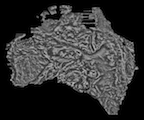
Surface Normals to Surfaces
 |
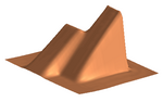 |
- shapeletsurf.m Function reconstructs an estimate of a surface from its surface normals by correlating the surface normals with that those of a bank of shapelet basis functions. The correlation results are summed to produce the reconstruction. The sumation of shapelet basis functions results in an implicit integration of the surface while enforcing surface continuity.
Note that the reconstruction is only valid up to a scale factor (which can be corrected for). However the reconstruction process is very robust to noise and to missing data values. Reconstructions (up to positive/negative shape ambiguity) are possible where there is an ambiguity of pi in tilt values. Low quality reconstructions are also possible with just slant, or just tilt data alone. However, if you have full gradient information you are better off with the Frankot Chellappa algorithm below.
- frankotchellappa.m An implementation of Frankot and Chellappa's algorithm for constructing an integrable surface from gradient information. If you have full gradient information in x and y this is probably the best algorithm to use. It is very simple, very fast and highly robust to noise. If you have surface normal information in the form of slant and tilt, and you have an ambiguity of pi in your tilt data, or only have slant, then try using shapeltsurf.m above.
- grad2slanttilt.m Converts gradient values over a surface to slant and tilt angles.
- slanttilt2grad.m Converts slant and tilt angles over a surface to gradients.
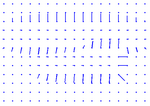
- needleplotgrad.m Generates a needle plot given surface gradients over a surface.
- needleplotst.m Generates a needle plot given slant and tilt values over a surface.
- testp.m Generates a synthetic test surface along with its surface normals for testing shapeletsurf.
Reference:
- Peter Kovesi, "Shapelets Correlated with Surface Normals Produce Surfaces". 10th IEEE International Conference on Computer Vision. Beijing. pp 994-1001. 2005
- PowerPoint Slides
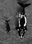
- An example of how much 3D shape you can get from very minimal surface normal information.
Scalogram Calculation
- scalogram.m Function to calculate the phase and amplitude scalograms of a 1D signal. The analysis is done using quadrature pairs of log Gabor wavelets.
Anisotropic diffusion

- anisodiff.m Function to perform anisotropic diffusion of an image following Perona and Malik's algorithm. This process smoothes regions while preserving, and enhancing, the contrast at sharp intensity gradients.
Grey Scale Transformation and Enhancement
- extractfields.m separates fields from a video frame, and optionally interpolates intermediate lines.
- interpfields.m interpolates lines on a field extracted from a video frame.
- normalise.m rescales image values to 0-1.
- adjcontrast.m adjusts image contrast using sigmoid function.
- adjgamma.m adjusts image gamma.
- greytrans.m allows you to interactively remap intensity values in a colour or greyscale image via a mapping function defined by a series of spline points. A feeble attempt at replicating xv's intensity mapping tool. It is not as fast but it does operate on floating point images allowing you to better preserve image fidelity. (Needs remapim.m).
- remapim.m is a non-interactive version of greytrans that allows you to apply an intensity mapping to a colour or greyscale image using a mapping function determined experimentally with greytrans. Useful if you want to apply the same mapping function to a sequence of images.
- histtruncate.m truncates ends of an image histogram. Useful for enhancing images with outlying values.
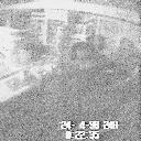
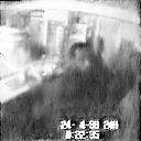
- histeqfloat.m This function differs from classical histogram equalisation functions in that the cumulative histogram treated as a function rather than as a lookup table for mapping input grey values to their output values. Under this approach, for images containing floating point values, the number of distinct values in the output image will be the same as the number of distinct values in the input. This can make a significant difference.
- Example of using some of these functions above to enhance a video surveillance image. However you should note that many surveillance systems are close to being legally blind. See
- Kovesi, P. Video Surveillance: Legally Blind? In Digital Image Computing: Techniques and Applications, 2009. DICTA '09. pp. 204-211.
IEEE Publishing. doi.org/10.1109/DICTA.2009.41
(preprint)
Frequency Domain Transformations
- perfft2.m 2D Fourier transform of the periodic component of Moisan's "Periodic plus Smooth Image Decomposition". I think this will become my default fft function for images.
- lowpassfilter.m constructs low-pass Butterworth filter.
- highpassfilter.m constructs high-pass Butterworth filter.
- highboostfilter.m constructs high-boost Butterworth filter.
- bandpassfilter.m constructs band-pass Butterworth filter.
- homomorphic.m performs homomorphic filtering on an image. One of my favourite image enhancement techniques. (needs histtruncate.m and normalise.m)
- psf.m generates a variety of point-spread functions. This function can be useful when manually specifying point-spread functions for Wiener filtering or with deconvolution functions such as the Richardson-Lucy algorithm (see the MATLAB Image Processing Toolbox function deconvlucy.m).
- psf2.m is identical to psf, it just has a different way of specifying the function shape which may be more convenient for some applications.
- imspect.m plots image amplitude spectrum averaged over all orientations.
- freqcomp.m demonstrates image reconstruction from its Fourier components.
- filtergrid.m Generates grid for constructing frequency domain filters. Used by some of the functions above.
For those working in Julia the package ImagePhaseCongruency.jl implements most of the functions above.
Functions Supporting Projective Geometry
 |
 |
- homography1d.m computes the 2x2 1D homography of 3 or more points along a line.
- homography2d.m computes the 3x3 2D homography of 4 or more points in a plane. This code follows the normalised direct linear transformation algorithm given by Hartley and Zisserman.
- fundmatrix.m computes the fundamental matrix from 8 or more matching points in a stereo pair of images using the normalised 8 point algorithm.
- affinefundmatrix.m computes the affine fundamental matrix from 4 or more matching points in a stereo pair of images.
- fundfromcameras.m computes fundamental matrix given two camera projection matrices.
- decomposecamera.m decomposes camera projection matrix into intrinsic and extrinsic parameters.
- rq3.m RQ decomposition of 3 x 3 matrix.
- skew.m Constructs 3x3 skew-symmetric matrix from a 3-vector.
- normalise2dpts.m translates and normalises a set of 2D homogeneous points so that their centroid is at the origin and their mean distance from the origin is sqrt(2). This is used to improve the conditioning of any equations used to solve homographies, fundamental matrices etc.
- hnormalise.m normalises an array of homogeneous coordinates so that their scale parameter is 1. Points at infinity are unchanged.
- makehomogeneous.m converts an N x npts array of inhomogeneous points to homogeneous points with scale 1.
- makeinhomogeneous.m normalises an N x npts array of homogeneous points to a scale of 1 and returns the inhomogeneous coordinates.
- ray2raydist.m computes shortest distance between two 3D rays.
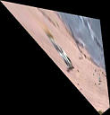
- imTrans.m applies a homogeneous transform to an image. The output image origin and size is adjusted to contain the transformed image. (Note I wrote this code before version 3 of the Image Processing Toolbox was released with the function IMTRANSFORM. You are probably better off using MATLAB's IMTRANSFORM)
- imTransD.m applies a homogeneous transform to an image. No origin shift is applied to the transformed image. I use this function for registering images etc.
- digiplane.m allows you to digitise and transform points within a planar region in an image.
- equalAngleConstraint.m Affine transform constraints given two equal angles.
- knownAngleConstraint.m Affine transform constraints given a known angle.
- lengthRatioConstraint Affine transform constraints given a length ratio.
- circleintersect.m Finds intersection of two circles. Use this function to solve for affine transformation constraints.
- hcross.m Homogeneous cross product, result normalised to s = 1.
- hline.m Plot 2D lines defined in homogeneous coordinates.
- homoTrans 2D homogeneous transformation of points/lines.
- plotPoint.m Plots point with specified mark and optional text label.
- cameraproject.m Projects 3D world points into a camera image.
- idealimagepts.m Computes image locations that would be obtained if the camera had no lens distortion.
- imagept2plane.m Projects image points to a plane and returns their 3D locations.
- solvestereopt.m Solves 3D location of a point given image coordinates of that point in two, or more, images.
- undistortimage.m Removes lens distortion from an image given the radial lens distortion coefficients.
- camstruct.m constructs a structure that holds camera parameters. These include lens distortion parameters and the image size.
- camstruct2projmatrix.m converts a camera structure to a 3x4 projection matrix ignoring lens distortion parameters.
- plotcamera.m Plots a representation of a camera in 3 space given a camera structure.
- If you are using these functions above you should look at Andrew Zisserman's MATLAB Functions for Multiple View Geometry
Also, you must listen to The Fundamental Matrix Song by Daniel Wedge.
For those working in Julia the package ImageProjectiveGeometry.jl implements most of the functions above.
Feature Matching
- matchbycorrelation.m generates putative matches between previously detected feature points in two images by looking for points that are maximally correlated with each other within windows surrounding each point. Only points that correlate most strongly with each other in both directions are returned. This is a simple-minded N2 comparison.
- matchbymonogenicphase.m is similar to matchbycorrelation, but instead matches on oriented phase values rather than greyscale values. This matcher performs rather well relative to normalised greyscale correlation. Typically there are more putative matches found and fewer outliers. There is a greater computational cost in the pre-filtering stage but potentially the matching stage is much faster as each pixel is effectively encoded with only 3 bits. (Though this potential speed is not realized in this implementation). See testfund below to see an example of the use of this function.
Model Fitting and Robust Estimation
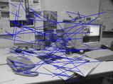 Putative matches obtained by matchbycorrelation.m |
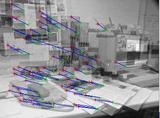 Inlying matches consistent with fundamental matrix |
- ransac.m a general purpose implementation of the RANSAC algorithm.
- ransacfithomography.m robustly fits a homography to a set of putatively matched image points.
- ransacfitfundmatrix.m robustly fits a fundamental matrix to a set of putatively matched image points. This function uses an 8 point fundamental matrix solution.
- ransacfitfundmatrix7.m robustly fits a fundamental matrix to a set of putatively matched image points. This function requires Andrew Zisserman's 7 point fundamental matrix code available from: MATLAB Functions for Multiple View Geometry
- ransacfitaffinefund.m robustly fits an affine fundamental matrix to a set of putatively matched image points.
- ransacfitplane.m robustly fits a plane to 3D data points.
- ransacfitline.m robustly fits a line to 3D data points.
- iscolinear.m tests if 3 points are colinear, used by ransacfitplane and ransacfithomography.
- fitline.m least squares fit of a line to 2D data points.
- fitline3d.m least squares fit of a line to 3D data points. Contributed by Felix Duvallet.
- fitplane.m least squares fit of a plane to 3D data points.
- testfitplane example of using ransacfitplane.m
- testfitline example of using ransacfitline.m
- testfund example of using ransacfitfundmatrix.m
- testhomog example of using ransacfithoography.m
- randomsample a basic replacement for randsample to be used with ransac.m should you not have the MATLAB Statistics Toolbox, or are using Octave.
- Example of using these functions above to find the fundamental matrix.
References:
- Listen to The RANSAC Song by Daniel Wedge.
- You should also check out his 2.71828183: The Number e Song
For those working in Julia the package ImageProjectiveGeometry.jl implements most of the functions above.
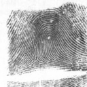
Fingerprint Enhancement
 |
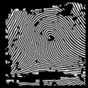 |
- ridgesegment.m identifies ridge-like regions of a fingerprint image. It also normalises the intensity values of the image.
- ridgeorient.m estimates the local orientation of ridges in a fingerprint.
- plotridgeorient.m plots ridge orientations calculated by ridgeorient.
- ridgefreq.m estimates the local ridge frequency across a fingerprint image.
- freqest.m estimates the ridge frequency within a small block of an image. This is used by ridgefreq.
- ridgefilter.m enhances a fingerprint image using oriented filters.
- Example of using these functions above.
Geoscientific and Geophysical Functions

- ppdrc.m Phase Preserving Dynamic Range Compression. A frequency based tonemapping algorithm suited to scientific, non-photographic images. Try using this function instead of histogram equalization. Very good on aeromagentic data. Requires highpassmonogenic.m
For those working in Julia the package ImagePhaseCongruency.jl provides an implementation of this function. - irelief.m Function for interactive relief shading of a dataset. Requires applycolourmap.m
- relief.m Non-interactive version of the function above.
- upwardcontinue.m Generates upward continuation of magnetic or gravity potential field data.
- freqderiv.m Horizontal and vertical derivatives computed via the frequency domain.
- vertderivativeintegral.m Vertical derivative or integral of potential field data.
- tiltderiv.m Generates tilt derivative of potential field data.
- analyticsignal.m Analytic signal of potential field data.
- agc.m This function implements Rajagopalan's Automatic Gain Control algorithm. The original application was for displaying geoscientific vertical magnetic gradient data but it can be useful for any kind of high dynamic range image.
- terrace.m This function implements a modified version of Cordell and McCafferty's terracing algorithm for potential field data. Its key attribute is that the output remains stable no matter how many iterations are applied.
- orientationfilter.m Generates orientation selective filterings of an image. Use for highlighting structures with dominant orientations in your data.
- dealias.m Filters an image in order to try to remove aliasing artifacts from any gridding process.
- wavenumbergrid.m Generate a wavenumber grid for frequency domain filtering.
- removetrend.m Fits a polynomial trend surface to a grid and removes it.
Reference:
- Peter Kovesi, "Phase Preserving Tone Mapping of Non-Photographic High Dynamic Range Images". Proceedings: The Australian Pattern Recognition Society Conference: Digital Image Computing: Techniques and Applications DICTA 2012. (preprint)
Interesting Synthetic and Test Images
- noiseonf.m generates noise images with specified amplitude spectra. One can create pleasing cloud pattern images this way.
- cloud9.m creates a movie sequence of noise images with specified amplitude spectra. Very relaxing.
- chirpexp.m creates an exponential chirp test image. The amplitude of the chirp is modulated from 1 at the top of the image to 0 at the bottom. I have used this test image to evaluate the effectiveness of different colourmaps, and sections of colourmaps, over varying spatial frequencies and contrast.
- chirplin.m similar to chirpexp.m but with a linear chirp signal.
- sineramp.m Generates a test image consisting of a sine wave superimposed on a ramp function The amplitude of the sine wave is modulated from its full value at the top of the image to 0 at the bottom. A useful test image for highlighting problems in colour maps.
- circlesineramp.m Generates a test image representing a cyclic version of sineramp.m for testing of cyclic colour maps. It consists of a sine wave superimposed on a spiral ramp function.
- derespolar.m Generates deresolved images in polar coordinates.
- polartrans.m Generates a polar transformation of an image. A linear or logarithmic radius transformation can be specified.
- quantizephase.m Generates an image where the phase values are quantized to a desired number of levels. Phase values in an image are important. However, despite this, they can be quantized very heavily with relatively little perceptual loss.
ASCII Image Generation
- matscii.m Function to generate ASCII images from grey scale images. A bit of retro fun, but constant width fonts are getting hard to come by these days...
Homogeneous Transforms
- plotframe.m plots a coordinate frame specified by a homogeneous transform.
- trans.m homogeneous tranlation matrix.
- rotx.m homogeneous matrix for rotation about x-axis.
- roty.m homogeneous matrix for rotation about y-axis.
- rotz.m homogeneous matrix for rotation about z-axis.
- homotrans.m homogeneous transformation of points/lines
- invht.m optimized inverse of homogeneous transformation matrix
- inveuler.m solves for euler angles given a homogeneous transform.
- invrpy.m solves for roll, pitch, yaw angles given a homogeneous transform.
- dhtrans.m calculates the 4x4 homogeneous Denavit Hartenberg matrix given link parameters of joint angle, length, joint offset, and twist.
Quaternions
- newquaternion.m construct quaternion from specified angle and axis.
- matrix2quaternion.m converts 4x4 homogeneous rotation matrix to quaternion
- quaternion2matrix.m converts quaternion to a 4x4 homogeneous transformation matrix.
- quaternionrotate.m uses quaternion to rotate vectors.
- quaternionproduct.m computes quaternion product.
- quaternionconjugate.m computes quaternion conjugate.
- vector2quaternion.m embeds a 3-vector in a quaternion.
Angle-Axis Descriptors
- newangleaxis.m constructs angle-axis descriptor from specified angle and axis.
- matrix2angleaxis.m converts homogeneous rotation matrix to angle-axis description
- angleaxis2matrix.m converts angle-axis descriptor to 4x4 homogeneous transformation matrix.
- angleaxisrotate.m uses angle axis descriptor to rotate vectors
- normaliseangleaxis.m normalises angle-axis descriptor so that the angle has a maximum magnitude of pi.
For those working in Julia the package ImageProjectiveGeometry.jl implements most of the functions above.
Image Display, Image Writing and Miscellaneous
- findimage.m Displays a file dialog box to allow you to find and load an image interactively. Useful when you have forgotten the name of your image, or can't be bothered typing it out.
- findimages.m Allows you to select and load multiple images. These are returned in a cell array.
- show.m Updated April 2018 This function conveniently displays an image with the right size, colors, range, and with a title. The figure window is sized to match the image, leaving no border, saving desktop real estate. Where possible the image is displayed as 'TrueSize', that is, pixels on the screen match pixels in the image.
- showangularim.m This function displays an image of angular data with a specified colour map. For angular data to be rendered correctly it is important that the data values are respected so that data values are correctly assigned to specific entries in a cyclic colour map. The assignment of values to colours also depends on whether the data is cyclic over pi, or 2*pi. This function also allows the colour map encoding of the angular information to be modulated to represent the amplitude/reliability/coherence of the angular data.
- showdivim.m This function is intended for displaying an image with a diverging colour map. To do this correctly requires that the desired reference value in the data is correctly associated with the centre entry of the diverging colour map.
- orientationplot.m Visualizes an orientation image with dithered oriented lines. The oriented line segments are plotted in a dithered grid pattern across the image. Use of a randomly dithered grid locations rather than a regular grid ensures that the grid pattern not interfere with your perception of the orientations. This improves the perception of the orientation pattern significantly.
- showfft.m displays the amplitude spectrum of an fft.
- showlogfft.m displays the log amplitude spectrum of an fft.
- showsurf.m This function wraps up the commands I usually use to display a surface. The surface is displayed using SURFL with interpolated shading, using the 'copper' colour map, with rotate3d on, and axis vis3d set.
- togglefigs.m provides a convenient means of toggling the display of multiple figures. Handy for comparing images and plots. The axes of the images are linked so that pan and zoom are synchronised on all images.
- New syncshow.m Show multiple images with axes linked for pan and zoom, or link a set of existing figures so that pan and zoom are synchronised.
- imwritesc.m This function combines image rescaling and writing into the one function. If the image type is double image values are rescaled to the range 0-1 so that no overflow occurs when writing 8-bit intensity values. The image format to use is determined by MATLAB from the file ending. If the image type is of uint8 no rescaling is performed.
- New imwritefloattiff.m This function makes use of Tiff, MATLAB's gateway to the LibTIFF library routines to provide a basic floating point image writing function. (MATLAB's imwrite() only seems to be able to write integer valued tiff images.)
- matprint.m This function prints out a matrix using a specified C style format string. Often you find that MATLAB's default number formats are not what you want...
- digipts.m Function to digitise points in an image. This function uses the cross-hair cursor provided by GINPUT. I find this is much more useable than the cursor used by IMPIXEL. In addition each location digitised is marked with a red '+'.
- impad Pads the boundary of an image prior to filtering. Various padding options available.
- imtrim Trims the boundary of an image (unpads it)
- imsetborder Sets border pixels of an image to a specified value.
- removenan Replaces NaN values in a matrix with a specified default value. Useful when you want to prevent NaNs from contaminating and destroying some operation on an array, for example, an FFT.
- fillnan Replaces NaN values in a matrix with the value in the closest non-Nan pixel.
- implace.m Function to place an image at a specified location within a larger image.
- cubicroots.m computes the real roots of a cubic.
- weightedhistc.m basic equivalent to MATLAB's HISTC function for weighted data.
- geoseries.m convenience function for generating geometric series.
- circle.m Draws a circle.
- circularstruct.m generates a circular structuring element for morphological operations. You can use MATLAB's strel('disk',R,0) instead. However occasionally I like being able to tweak the shape by using floating point values for the radius.
- pointinconvexpoly.m Determine if a 2D point is within a convex polygon.
- rectintersect.m Determine if two rectangles intersect.
- polyfit2d.m Fits 2D polynomial surface to data. Basic 2D equivalent of MATLAB's 1D polyfit. Incorporates some normalisation to reduce numerical problems.
- polyval2d.m Evaluates 2D polynomial surface generated by polyfit2d.m
- logcolournormalization.m Perform chromaticity, grey, or comprehensive colour normalization on a colour image.
- svddemo.m Demonstration of the SVD and eigenvalues for a 2x2 transformation matrix.
Geometric shapes
- icosahedron.m generates the vertices, adjacency graph and face list of an icosahedron.
- geodome.m generates the vertices, adjacency graph and face list of a geodesic sphere. Apart from looking cool the vertices, or face centres, of a geodesic sphere can be useful for defining the bin centres of a 3D orientation histogram.
- gplot3d.m a 3D version of MATLAB's gplot function.
- drawfaces.m draws triangular faces defined by a set of vertices and a corresponding face vertex list.
- superquad.m generates parametric surfaces of superquadratics.
- supertorus.m generates parametric surfaces of a supertorus.
String handling convenience functions
- strstartswith.m tests if a string starts with a specified substring.
- strendswith.m tests if a string ends with a specified substring.
- namenpath.m returns filename and its path from a full filename that may include a directory path
- basename.m trims off the suffix ending from a filename.
- pathlist.m produces a cell array of directories along a directory path