Introduction
Often we are interested in finding patterns which appear over a space of time. These patterns occur in many areas; the pattern of commands someone uses in instructing a computer, sequences of words in sentences, the sequence of phonemes in spoken words - any area where a sequence of events occurs could produce useful patterns.
Consider the simple example of someone trying to deduce the weather from a piece of seaweed - folklore tells us that `soggy’ seaweed means wet weather, while `dry’ seaweed means sun. If it is in an intermediate state (`damp’), then we cannot be sure. However, the state of the weather is not restricted to the state of the seaweed, so we may say on the basis of an examination that the weather is probably raining or sunny. A second useful clue would be the state of the weather on the preceding day (or, at least, its probable state) - by combining knowledge about what happened yesterday with the observed seaweed state, we might come to a better forecast for today.
This is typical of the type of system we will consider in this tutorial.
- First we will introduce systems which generate probabalistic patterns in time, such as the weather fluctuating between sunny and rainy.
- We then look at systems where what we wish to predict is not what we observe - the underlying system is hidden. In the above example, the observed sequence would be the seaweed and the hidden system would be the actual weather.
- We then look at some problems that can be solved once the system has been modeled. For the above example, we may want to know
- What the weather was for a week given each day’s seaweed observation.
- Given a sequence of seaweed observations, is it winter or summer? Intuitively, if the seaweed has been dry for a while it may be summer, if it has been soggy for a while it might be winter.
Generating Patterns
Deterministic Non-Deterministic Summary Section 1 - Page 1 Deterministic Patterns
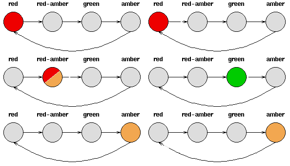
Consider a set of traffic lights; the sequence of lights isred - red/amber - green - amber - red. The sequence can be pictured as a state machine, where the different states of the traffic lights follow each other.
Notice that each state is dependent solely on the previous state, so if the lights are green, an amber light will always follow - that is, the system is deterministic. Deterministic systems are relatively easy to understand and analyse, once the transitions are fully known.
Generating Patterns
Deterministic Non-Deterministic Summary Section 2 - Page 1
1 2 3 4Non-deterministic patterns
To make the weather example a little more realistic, introduce a third state - cloudy. Unlike the traffic light example, we cannot expect these three weather states to follow each other deterministically, but we might still hope to model the system that generates a weather pattern.
One way to do this is to assume that the state of the model depends only upon the previous states of the model. This is called the Markov assumption and simplifies problems greatly. Obviously, this may be a gross simplification and much important information may be lost because of it.
When considering the weather, the Markov assumption presumes that today’s weather can always be predicted solely given knowledge of the weather of the past few days - factors such as wind, air pressure etc. are not considered. In this example, and many others, such assumptions are obviously unrealistic. Nevertheless, since such simplified systems can be subjected to analysis, we often accept the assumption in the knowledge that it may generate information that is not fully accurate.
Section 2 - Page 2
1 2 3 4
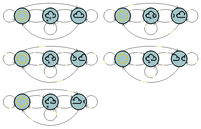
A Markov process is a process which moves from state to state depending (only) on the previous n states. The process is called an order n model where n is the number of states affecting the choice of next state. The simplest Markov process is a first order process, where the choice of state is made purely on the basis of the previous state. Notice this is not the same as a deterministic system, since we expect the choice to be made probabalistically, not deterministically.The figure below shows all possible first order transitions between the states of the weather example.
Notice that for a first order process with M states, there are M2 transitions between states since it is possible for any one state to follow another. Associated with each transition is a probability called the state transition probability - this is the probability of moving from one state to another. These M2 probabilities may be collected together in an obvious way into a state transition matrix. Notice that these probabilities do not vary in time - this is an important (if often unrealistic) assumption.
Section 2 - Page 3
1 2 3 4
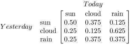
The state transition matrix below shows possible transition probabilities for the weather example;
- that is, if it was sunny yesterday, there is a probability of 0.5 that it will be sunny today, and 0.375 that it will be cloudy. Notice that (because the numbers are probabilities) the sum of the entries for each row is 1.
Section 2 - Page 4
1 2 3 4
To initialise such a system, we need to state what the weather was (or probably was) on the day after creation; we define this in a vector of initial probabilities, called the vector.
- that is, we know it was sunny on day 1.
We have now defined a first order Markov process consisting of :
- states : Three states - sunny, cloudy, rainy.
 vector : Defining the probability of the system being in each of the states at time 0.
- state transition matrix : The probability of the weather given the previous day’s weather.
Generating Patterns
Deterministic Non-Deterministic Summary Section 3 - Page 1 Summary
We are trying to recognise patterns in time, and in order to do so we attempt to model the process that could have generated the pattern. We use discrete time steps, discrete states, and we may make the Markov assumption. Having made these assumptions, the system producing the patterns can be described as a Markov process consisting of a
 vector and a state transition matrix.
An important point about the assumption is that the state transition probabilites do not vary in time - the matrix is fixed throughout the life of the system.
vector and a state transition matrix.
An important point about the assumption is that the state transition probabilites do not vary in time - the matrix is fixed throughout the life of the system.Patterns generated by a hidden process
Limitations of a Markov Process Hidden Markov Models Summary Section 1 - Page 1
1 2When a Markov process may not be powerful enough
In some cases the patterns that we wish to find are not described sufficiently by a Markov process. Returning to the weather example, a hermit may perhaps not have access to direct weather observations, but does have a piece of seaweed. Folklore tells us that the state of the seaweed is probabalistically related to the state of the weather - the weather and seaweed states are closely linked. In this case we have two sets of states, the observable states (the state of the seaweed) and the hidden states (the state of the weather). We wish to devise an algorithm for the hermit to forecast weather from the seaweed and the Markov assumption without actually ever seeing the weather.A more realistic problem is that of recognising speech; the sound that we hear is the product of the vocal chords, size of throat, position of tongue and several other things. Each of these factors interact to produce the sound of a word, and the sounds that a speech recognition system detects are the changing sound generated from the internal physical changes in the person speaking.
Section 1 - Page 2
1 2
Some speech recognition devices work by considering the internal speech production to be a sequence of hidden states, and the resulting sound to be a sequence of observable states generated by the speech process that at best approximates the true (hidden) states. In both examples it is important to note that the number of states in the hidden process and the number of observable states may be different. In a three state weather system (sunny, cloudy, rainy) it may be possible to observe four grades of seaweed dampness (dry, dryish, damp,soggy); pure speech may be described by (say) 80 phonemes, while a physical speech system may generate a number of distinguishable sounds that is either more or less than 80.In such cases the observed sequence of states is probabalistically related to the hidden process. We model such processes using a hidden Markov model where there is an underlying hidden Markov process changing over time, and a set of observable states which are related somehow to the hidden states.
Patterns generated by a hidden process
Limitations of a Markov Process Hidden Markov Models Summary Section 2 - Page 1
1 2Hidden Markov Models
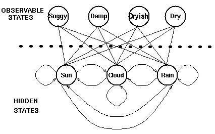
The diagram below shows the hidden and observable states in the weather example. It is assumed that the hidden states (the true weather) are modelled by a simple first order Markov process, and so they are all connected to each other.
Section 2 - Page 2
1 2The connections between the hidden states and the observable states represent the probability of generating a particular observed state given that the Markov process is in a particular hidden state. It should thus be clear that all probabilities `entering’ an observable state will sum to 1, since in the above case it would be the sum ofPr(Obs|Sun), Pr(Obs|Cloud) and Pr(Obs|Rain).
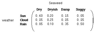
In addition to the probabilities defining the Markov process, we therefore have another matrix, termed the confusion matrix, which contains the probabilities of the observable states given a particular hidden state. For the weather example the confusion matrix might be;
Notice that the sum of each matrix row is 1.
Patterns generated by a hidden process
Limitations of a Markov Process
Hidden Markov Models
Summary
Section 3 - Page 1
1 2
Summary
We have seen that there are some processes where an observed sequence is probabalistically related to an underlying Markov process. In such cases, the number of observable states may be different to the number
of hidden states.We model such cases using a hidden Markov model (HMM). This is a model containing two sets of states and three sets of probabilities;
- hidden states : the (TRUE) states of a system that may be described by a Markov process (e.g., the weather).
- observable states : the states of the process that are `visible’ (e.g., seaweed dampness).
1 2
 vector : contains the probability of the (hidden) model being in a particular hidden state at time t = 1.
- state transition matrix : holding the probability of a hidden state given the previous hidden state.
- confusion matrix : containing the probability of observing a particular observable state given that the hidden model is in a particular hidden state.
Thus a hidden Markov model is a standard Markov process augmented by a set of observable states, and some probabalistic relations between them and the hidden states.
Forward Algorithm
| |
|
|
|
1 2 3 4 5 6 7 8 9 10 11 12
Finding the probability of an observed sequence
1. Exhaustive search for solution
We want to find the probability of an observed sequence given an HMM - that is, the parameters ( ,A,B)
,A,B)
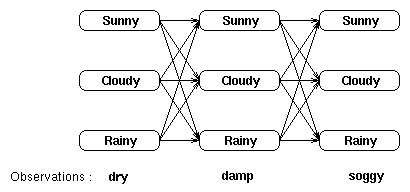
are known. Consider the weather example; we have a HMM describing the weather and its relation to the state of the seaweed, and we also have a sequence of seaweed observations. Suppose the observations for 3 consecutive days are (dry,damp,soggy) - on each
of these days, the weather may have been sunny, cloudy or rainy. We can picture the observations and the possible hidden states as a trellis.
1 2 3 4 5 6 7 8 9 10 11 12
Each column in the trellis shows the possible state of the weather and each state in one column is connected to each state in the adjacent columns. Each of these state transitions has a probability provided by
the state transition matrix. Under each column is the observation at that time; the probability of this observation given any one of the above states is provided by the confusion matrix.
It can be seen that one method of calculating the probability of the observed sequence would be to find each possible sequence of the hidden states, and sum these probabilities. For the above example, there would be 3^3=27 possible different weather sequences, and so the probability is
Pr(dry,damp,soggy | HMM) = Pr(dry,damp,soggy | sunny,sunny,sunny) + Pr(dry,damp,soggy | sunny,sunny ,cloudy) + Pr(dry,damp,soggy | sunny,sunny ,rainy) + … . Pr(dry,damp,soggy | rainy,rainy ,rainy)
Calculating the probability in this manner is computationally expensive, particularly with large models or long sequences, and we find that we can use the time invariance of the probabilities to reduce the complexity of the problem.
1 2 3 4 5 6 7 8 9 10 11 12
2. Reduction of complexity using recursion
We will consider calculating the probability of observing a sequence recursively given a HMM. We will first define a partial probability, which is the probability of reaching an intermediate state in the trellis.
We then show how these partial probabilities are calculated at times t=1 and t=n (> 1).
Suppose throughout that the T-long observed sequence is
2a. Partial probabilities, ( ’s)
’s)
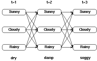
Consider the trellis below showing the states and first-order transitions for the observation sequence dry,damp,soggy;
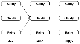
We can calculate the probability of reaching an intermediate state in the trellis as the sum of all possible paths to that state.For example, the probability of it being cloudy at t = 2 is calculated from the paths;
We denote the partial probability of state j at time t ast ( j ) - this partial probability is calculated as;
t ( j )= Pr( observation | hidden state is j ) x Pr(all paths to state j at time t)
The partial probabilities for the final observation hold the probability of reaching those states going through all possible paths - e.g., for the above trellis, the final partial probabilities are calculated from the paths :
It follows that the sum of these final partial probabilities is the sum of all possible paths through the trellis, and hence is the probability of observing the sequence given the HMM.Section 3 introduces an animated example of the calculation of the probabilities.
