BP算法演示 - 润新知

BP算法演示

本文转载自https://mattmazur.com/2015/03/17/a-step-by-step-backpropagation-example/

Background

Backpropagation is a common method for training a neural network. There is no shortage of papers online that attempt to explain how backpropagation works, but few that include an example with actual numbers. This post is my attempt to explain how it works with a concrete example that folks can compare their own calculations to in order to ensure they understand backpropagation correctly.

If this kind of thing interests you, you should sign up for my newsletter where I post about AI-related projects that I’m working on.

Backpropagation in Python

You can play around with a Python script that I wrote that implements the backpropagation algorithm in this Github repo.

Backpropagation Visualization

For an interactive visualization showing a neural network as it learns, check out my Neural Network visualization.

Additional Resources

If you find this tutorial useful and want to continue learning about neural networks and their applications, I highly recommend checking out Adrian Rosebrock’s excellent tutorial on Getting Started with Deep Learning and Python.

Overview

For this tutorial, we’re going to use a neural network with two inputs, two hidden neurons, two output neurons. Additionally, the hidden and output neurons will include a bias.

Here’s the basic structure:

In order to have some numbers to work with, here are the initial weights, the biases, and training inputs/outputs:

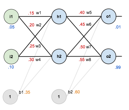
The goal of backpropagation is to optimize the weights so that the neural network can learn how to correctly map arbitrary inputs to outputs.

For the rest of this tutorial we’re going to work with a single training set: given inputs 0.05 and 0.10, we want the neural network to output 0.01 and 0.99.

The Forward Pass

To begin, lets see what the neural network currently predicts given the weights and biases above and inputs of 0.05 and 0.10. To do this we’ll feed those inputs forward though the network.

We figure out the total net input to each hidden layer neuron, squash the total net input using an activation function (here we use the logistic function), then repeat the process with the output layer neurons.

Total net input is also referred to as just net input by some sources.

Here’s how we calculate the total net input for $h_1$ :

$net_{h1} = w_1 * i_1 + w_2 * i_2 + b_1 * 1$

$net_{h1} = 0.15 * 0.05 + 0.2 * 0.1 + 0.35 * 1 = 0.3775$

We then squash it using the logistic function to get the output of $h_1$ :

$out_{h1} = frac{1}{1+e^{-net_{h1}}} = frac{1}{1+e^{-0.3775}} = 0.593269992$

Carrying out the same process for $h_2$ we get:

$out_{h2} = 0.596884378$

We repeat this process for the output layer neurons, using the output from the hidden layer neurons as inputs.

Here’s the output for $o_1$ :

$net_{o1} = w_5 * out_{h1} + w_6 * out_{h2} + b_2 * 1$

$net_{o1} = 0.4 * 0.593269992 + 0.45 * 0.596884378 + 0.6 * 1 = 1.105905967$

$out_{o1} = frac{1}{1+e^{-net_{o1}}} = frac{1}{1+e^{-1.105905967}} = 0.75136507$

And carrying out the same process for $o_2$ we get:

$out_{o2} = 0.772928465$

Calculating the Total Error

We can now calculate the error for each output neuron using the squared error function and sum them to get the total error:

$E_{total} = sum frac{1}{2}(target - output)^{2}$

Some sources refer to the target as the ideal and the output as the actual.

The $frac{1}{2}$ is included so that exponent is cancelled when we differentiate later on. The result is eventually multiplied by a learning rate anyway so it doesn’t matter that we introduce a constant here [1].

For example, the target output for $o_1$ is 0.01 but the neural network output 0.75136507, therefore its error is:

$E_{o1} = frac{1}{2}(target_{o1} - out_{o1})^{2} = frac{1}{2}(0.01 - 0.75136507)^{2} = 0.274811083$

Repeating this process for $o_2$ (remembering that the target is 0.99) we get:

$E_{o2} = 0.023560026$

The total error for the neural network is the sum of these errors:

$E_{total} = E_{o1} + E_{o2} = 0.274811083 + 0.023560026 = 0.298371109$

The Backwards Pass

Our goal with backpropagation is to update each of the weights in the network so that they cause the actual output to be closer the target output, thereby minimizing the error for each output neuron and the network as a whole.

Output Layer

Consider $w_5$ . We want to know how much a change in $w_5$ affects the total error, aka $frac{partial E_{total}}{partial w_{5}}$ .

$frac{partial E_{total}}{partial w_{5}}$ is read as “the partial derivative of $E_{total}$ with respect to $w_{5}$ “. You can also say “the gradient with respect to $w_{5}$ “.

By applying the chain rule we know that:

$frac{partial E_{total}}{partial w_{5}} = frac{partial E_{total}}{partial out_{o1}} * frac{partial out_{o1}}{partial net_{o1}} * frac{partial net_{o1}}{partial w_{5}}$

Visually, here’s what we’re doing:

We need to figure out each piece in this equation.

First, how much does the total error change with respect to the output?

$E_{total} = frac{1}{2}(target_{o1} - out_{o1})^{2} + frac{1}{2}(target_{o2} - out_{o2})^{2}$

$frac{partial E_{total}}{partial out_{o1}} = 2 * frac{1}{2}(target_{o1} - out_{o1})^{2 - 1} * -1 + 0$

$frac{partial E_{total}}{partial out_{o1}} = -(target_{o1} - out_{o1}) = -(0.01 - 0.75136507) = 0.74136507$

$-(target - out)$ is sometimes expressed as $out - target$

When we take the partial derivative of the total error with respect to $out_{o1}$ , the quantity $frac{1}{2}(target_{o2} - out_{o2})^{2}$ becomes zero because $out_{o1}$ does not affect it which means we’re taking the derivative of a constant which is zero.

Next, how much does the output of $o_1$ change with respect to its total net input?

The partial derivative of the logistic function is the output multiplied by 1 minus the output:

$out_{o1} = frac{1}{1+e^{-net_{o1}}}$

$frac{partial out_{o1}}{partial net_{o1}} = out_{o1}(1 - out_{o1}) = 0.75136507(1 - 0.75136507) = 0.186815602$

Finally, how much does the total net input of $o1$ change with respect to $w_5$ ?

$net_{o1} = w_5 * out_{h1} + w_6 * out_{h2} + b_2 * 1$

$frac{partial net_{o1}}{partial w_{5}} = 1 * out_{h1} * w_5^{(1 - 1)} + 0 + 0 = out_{h1} = 0.593269992$

Putting it all together:

$frac{partial E_{total}}{partial w_{5}} = frac{partial E_{total}}{partial out_{o1}} * frac{partial out_{o1}}{partial net_{o1}} * frac{partial net_{o1}}{partial w_{5}}$

$frac{partial E_{total}}{partial w_{5}} = 0.74136507 * 0.186815602 * 0.593269992 = 0.082167041$

You’ll often see this calculation combined in the form of the delta rule:

$frac{partial E_{total}}{partial w_{5}} = -(target_{o1} - out_{o1}) * out_{o1}(1 - out_{o1}) * out_{h1}$

Alternatively, we have $frac{partial E_{total}}{partial out_{o1}}$ and $frac{partial out_{o1}}{partial net_{o1}}$ which can be written as $frac{partial E_{total}}{partial net_{o1}}$ , aka $delta_{o1}$ (the Greek letter delta) aka the node delta. We can use this to rewrite the calculation above:

$delta_{o1} = frac{partial E_{total}}{partial out_{o1}} * frac{partial out_{o1}}{partial net_{o1}} = frac{partial E_{total}}{partial net_{o1}}$

$delta_{o1} = -(target_{o1} - out_{o1}) * out_{o1}(1 - out_{o1})$

Therefore:

$frac{partial E_{total}}{partial w_{5}} = delta_{o1} out_{h1}$

Some sources extract the negative sign from $delta$ so it would be written as:

$frac{partial E_{total}}{partial w_{5}} = -delta_{o1} out_{h1}$

/*每个权重的梯度都等于与其相连的前一层节点的输出（即 $out_{o1}$ */

To decrease the error, we then subtract this value from the current weight (optionally multiplied by some learning rate, eta, which we’ll set to 0.5):

$w_5^{+} = w_5 - eta * frac{partial E_{total}}{partial w_{5}} = 0.4 - 0.5 * 0.082167041 = 0.35891648$

Some sources use $alpha$ (alpha) to represent the learning rate, others use $eta$ (eta), and others even use $epsilon$ (epsilon).

We can repeat this process to get the new weights $w_6$ , $w_7$ , and $w_8$ :

$w_6^{+} = 0.408666186$

$w_7^{+} = 0.511301270$

$w_8^{+} = 0.561370121$

We perform the actual updates in the neural network after we have the new weights leading into the hidden layer neurons (ie, we use the original weights, not the updated weights, when we continue the backpropagation algorithm below).

Hidden Layer

Next, we’ll continue the backwards pass by calculating new values for $w_1$ , $w_2$ , $w_3$ , and $w_4$ .

Big picture, here’s what we need to figure out:

$frac{partial E_{total}}{partial w_{1}} = frac{partial E_{total}}{partial out_{h1}} * frac{partial out_{h1}}{partial net_{h1}} * frac{partial net_{h1}}{partial w_{1}}$

Visually:

We’re going to use a similar process as we did for the output layer, but slightly different to account for the fact that the output of each hidden layer neuron contributes to the output (and therefore error) of multiple output neurons. We know that $out_{h1}$ affects both $out_{o1}$ and $out_{o2}$ therefore the $frac{partial E_{total}}{partial out_{h1}}$ needs to take into consideration its effect on the both output neurons:

$frac{partial E_{total}}{partial out_{h1}} = frac{partial E_{o1}}{partial out_{h1}} + frac{partial E_{o2}}{partial out_{h1}}$

Starting with $frac{partial E_{o1}}{partial out_{h1}}$ :

$frac{partial E_{o1}}{partial out_{h1}} = frac{partial E_{o1}}{partial net_{o1}} * frac{partial net_{o1}}{partial out_{h1}}$

We can calculate $frac{partial E_{o1}}{partial net_{o1}}$ using values we calculated earlier:

$frac{partial E_{o1}}{partial net_{o1}} = frac{partial E_{o1}}{partial out_{o1}} * frac{partial out_{o1}}{partial net_{o1}} = 0.74136507 * 0.186815602 = 0.138498562$

And $frac{partial net_{o1}}{partial out_{h1}}$ is equal to $w_5$ :

$net_{o1} = w_5 * out_{h1} + w_6 * out_{h2} + b_2 * 1$

$frac{partial net_{o1}}{partial out_{h1}} = w_5 = 0.40$

Plugging them in:

$frac{partial E_{o1}}{partial out_{h1}} = frac{partial E_{o1}}{partial net_{o1}} * frac{partial net_{o1}}{partial out_{h1}} = 0.138498562 * 0.40 = 0.055399425$

Following the same process for $frac{partial E_{o2}}{partial out_{h1}}$ , we get:

$frac{partial E_{o2}}{partial out_{h1}} = -0.019049119$

Therefore:

$frac{partial E_{total}}{partial out_{h1}} = frac{partial E_{o1}}{partial out_{h1}} + frac{partial E_{o2}}{partial out_{h1}} = 0.055399425 + -0.019049119 = 0.036350306$

Now that we have $frac{partial E_{total}}{partial out_{h1}}$ , we need to figure out $frac{partial out_{h1}}{partial net_{h1}}$ and then $frac{partial net_{h1}}{partial w}$ for each weight:

$out_{h1} = frac{1}{1+e^{-net_{h1}}}$

$frac{partial out_{h1}}{partial net_{h1}} = out_{h1}(1 - out_{h1}) = 0.59326999(1 - 0.59326999 ) = 0.241300709$

We calculate the partial derivative of the total net input to $h_1$ with respect to $w_1$ the same as we did for the output neuron:

$net_{h1} = w_1 * i_1 + w_2 * i_2 + b_1 * 1$

$frac{partial net_{h1}}{partial w_1} = i_1 = 0.05$

Putting it all together:

$frac{partial E_{total}}{partial w_{1}} = frac{partial E_{total}}{partial out_{h1}} * frac{partial out_{h1}}{partial net_{h1}} * frac{partial net_{h1}}{partial w_{1}}$

$frac{partial E_{total}}{partial w_{1}} = 0.036350306 * 0.241300709 * 0.05 = 0.000438568$

You might also see this written as:

$frac{partial E_{total}}{partial w_{1}} = (sumlimits_{o}{frac{partial E_{total}}{partial out_{o}} * frac{partial out_{o}}{partial net_{o}} * frac{partial net_{o}}{partial out_{h1}}}) * frac{partial out_{h1}}{partial net_{h1}} * frac{partial net_{h1}}{partial w_{1}}$

$frac{partial E_{total}}{partial w_{1}} = (sumlimits_{o}{delta_{o} * w_{ho}}) * out_{h1}(1 - out_{h1}) * i_{1}$

$frac{partial E_{total}}{partial w_{1}} = delta_{h1}i_{1}$

/*每个权重的梯度都等于与其相连的前一层节点的输出（即i1*/

We can now update $w_1$ :

$w_1^{+} = w_1 - eta * frac{partial E_{total}}{partial w_{1}} = 0.15 - 0.5 * 0.000438568 = 0.149780716$

Repeating this for $w_2$ , $w_3$ , and $w_4$

$w_2^{+} = 0.19956143$

$w_3^{+} = 0.24975114$

$w_4^{+} = 0.29950229$

Finally, we’ve updated all of our weights! When we fed forward the 0.05 and 0.1 inputs originally, the error on the network was 0.298371109. After this first round of backpropagation, the total error is now down to 0.291027924. It might not seem like much, but after repeating this process 10,000 times, for example, the error plummets to 0.000035085. At this point, when we feed forward 0.05 and 0.1, the two outputs neurons generate 0.015912196 (vs 0.01 target) and 0.984065734 (vs 0.99 target).

总结：

1、每个权重的梯度都等于与其相连的前一层节点的输出　　

3、参考博文：http://blog.csdn.net/zhongkejingwang/article/details/44514073
相关阅读:
SASL简单认证和安全框架
 最详细的git rebase解释文章
 基于钻孔数据的三维地质模型可视化
 数字孪生 3D 风电场，智慧风电之陆上风电
 石油储运生产 2D 可视化，组态应用赋能工业智慧发展
 在抽象类中使用@Autowired
vue点击复制
 利用PHPJWT实现token及刷新token
PHP win32service Windows 系统后台服务
 SeasLog PHP 日志扩展
原文地址：https://www.cnblogs.com/shuaishuaidefeizhu/p/6776357.html

Copyright © 2020-2023 润新知