机器学习算法--Perceptron(感知器)算法

概括

Perceptron(感知器)是一个二分类线性模型，其输入的是特征向量，输出的是类别。Perceptron的作用即将数据分成正负两类的超平面。可以说是机器学习中最基本的分类器。

模型

Perceptron 一样属于线性分类器。
对于向量(X={x}_1,{x}_2,...{x}_n)，对于权重向量（w）相乘，加上偏移（b），于是有：

[f(x) = sum_{i=1}^N w_i mathbf{x}_i+b ]

设置阈值threshold之后，可以的到

[如果 f(x) > threshold, 则 y(标签)设为1 ]

[如果 f(x) < threshold, 则 y(标签)设为0 ]

即，可以把其表示为：

[mathbf{y} = sign(mathbf{w}^{T} mathbf{x}+mathbf{b}) ]

参数学习

我们已经知道模型是什么样，也知道Preceptron有两个参数，那么如何更新这两个参数呢？
首先，我们先Preceptron的更新策略：

1. 初始化参数

2. 对所有数据进行判断，超平面是否可以把正实例点和负实例点完成正确分开。

3. 如果不行，更新w，b。

4. 重复执行2，3步，直到数据被分开，或者迭代次数到达上限。

那么如何更新w，b呢？

​ 我们知道在任何时候，学习是朝着损失最小的地方，也就是说，我的下一步更新的策略是使当前点到超平面的损失函数极小化。
​ 在超平面中，我们定义一个点到超平面的距离为：(具体如何得出，可以自行百度~~~ )，此外其中$ frac{1}{left | mathbf{w} ight |}$是L2范数。意思可表示全部w向量的平方和的开方。

[frac{1}{left | mathbf{w} ight |} left | mathbf{w}^{T} mathbf{x}+mathbf{b} ight | ]

这里假设有M个点是误差点，那么损失函数可以是：

[L(mathbf{w},mathbf{b}) = -frac{1}{left | mathbf{w} ight |}sum_{mathbf{x}_{i}in M}mathbf{y}_{i}(mathbf{w}^{T} mathbf{x}+mathbf{b}) ]

当然，为了简便计算，这里忽略$ frac{1}{left | mathbf{w} ight |}$。

• $ frac{1}{left | mathbf{w} ight |}$不影响-y(w,x+b)正负的判断，即不影响学习算法的中间过程。

• 因为感知机学习算法最终的终止条件是所有的输入都被正确分类，即不存在误分类的点。则此时损失函数为0，则可以看出$ frac{1}{left | mathbf{w} ight |}$对最终结果也无影响。

• 既然没有影响，为了简便计算，直接忽略$ frac{1}{left | mathbf{w} ight |}$。

  • 这里可以把损失函数表示为：

[L(mathbf{w},mathbf{b}) = -sum_{mathbf{x}_{i}in M}mathbf{y}_{i}(mathbf{w}^{T} mathbf{x}+mathbf{b}) ]

这里我们只对一个点到超平面的损失进行计算。利用(L(mathbf{w},mathbf{b}))分别对w跟b求导，可得使L最小的w，b：

[ L(mathbf{w},mathbf{b}) = -mathbf{y}_{i}(mathbf{w}^{T} mathbf{x}+mathbf{b})Rightarrow left{egin{matrix}frac{partial L(mathbf{w},mathbf{b})}{partial mathbf{w}} = -y_{i}x_{i}\frac{partial L(mathbf{w},mathbf{b})}{partial mathbf{b}} = -y_{i}end{matrix} ight. ]

那么对于w,b的更新可以表示为：

[w_{k+1} = w_{k}+y_{i}x_{i} ]

[b_{k+1} = b_{k}+y_{i} ]

注意

对于线性可分的数据，Perceptron在有限的迭代里一定会找到一个超平面，可以把数据正确分类，但是这个分离超平面不是唯一的。

对于线性不可分数据，Perceptron学习算法永远不会结束，只可能达到迭代次数，因为不存在超平面完美分类数据，学习后期的超平面会一直“震荡”。

验证及代码

首先生成一组数据，可以完美线性可分

import matplotlib.pyplot as plt
import numpy as np
%matplotlib inline

# generate the separable data
def generate_separable_data(N):
    np.random.seed(2333)  # for reproducibility
    w = np.random.uniform(-1, 1, 2)
    b = np.random.uniform(-1, 1)
    X = np.random.uniform(-1, 1, [N, 2])
    y = np.sign(np.inner(w, X)+b)
    return X,y,w,b

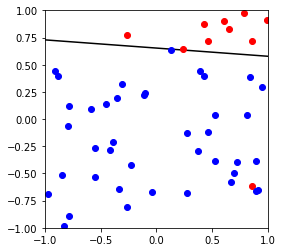
# generate the non separable data, set the first negative point as the positive point.
def generate_non_separable_data(N):
    np.random.seed(2333)  # for reproducibility
    w = np.random.uniform(-1, 1, 2)
    b = np.random.uniform(-1, 1)
    X = np.random.uniform(-1, 1, [N, 2])
    y = np.sign(np.inner(w, X)+b)
    for i in range(len(y)):
        if y[i] == -1:
            y[i] = 1
            break
            
    return X,y,w,b

#plot the data 
def plot_data(X, y, w, b) :
    fig = plt.figure(figsize=(4,4))
    plt.xlim(-1,1)
    plt.ylim(-1,1)
    a = -w[0]/w[1]
    pts = np.linspace(-1,1)
    plt.plot(pts, a*pts-(b/w[1]), 'k-')
    cols = {1: 'r', -1: 'b'}
    for i in range(len(X)): 
        plt.plot(X[i][0], X[i][1], cols[y[i]]+'o')
    plt.show()

X,y,w,b = generate_separable_data(50)
plot_data(X, y, w,b)

X,y,w,b = generate_non_separable_data(50)
plot_data(X, y, w,b)

The Perceptron

class Perceptron :
 
    """An implementation of the perceptron algorithm."""
 
    def __init__(self, max_iterations=100, learning_rate=0.2) :
 
        self.max_iterations = max_iterations
        self.learning_rate = learning_rate
 
    def fit(self, X, y) :
        X = self.add_bias(X,y)
        
        self.w = np.zeros(len(X[0]))

        converged = False
        iterations = 0
        while (not converged and iterations <= self.max_iterations) :
            converged = True
            for i in range(len(X)) :
                if y[i] * self.decision_function(X[i]) <= 0 :
                    self.w = self.w + y[i] * self.learning_rate * X[i]
                    converged = False
            iterations += 1
        self.converged = converged
        plot_data(X[:,1:], y, self.w[1:],self.w[0])
        if converged :
            print ('converged in %d iterations ' % iterations)
        else:
            print ('cannot converged in %d iterations ' % iterations)

        print ('weight vector: ' + str(self.w))

    def decision_function(self, x) :
        return np.inner(self.w, x)

    def predict(self, X) :
        scores = np.inner(self.w, X)
        return np.sign(scores)
    
    def add_bias(self,X,y):
        a = np.ones(X.shape[0])
        X = np.insert(X, 0, values=a, axis=1)
        return X
    def error(self,X,y):
        num = 0
        err_sco = self.predict(X)
        num =sum (err_sco!=y)
        return num/len(X)

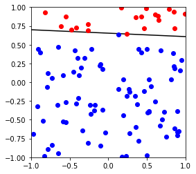
测试可以分割的数据

X,y,w,b = generate_separable_data(100)
p = Perceptron()
p.fit(X,y)

converged in 41 iterations 
weight vector: [-1.          0.07009608  1.53050105]

The Pocket

一种优化后的Perceptron。

Pocket 与Perceptron的参数更新一致，但是pocket在一定程度上解决了Perceptron震荡的问题。

• 在Perceptron中，碰到无法完美分割的数据集，只能等迭代次数到达上限，至于结果，无法预知，可能较好，可能很差，取决于震荡的结果。
• 而在Pocket中，我们加入了最优参数的记录，保证记录的参数是最好的，那么即使不能完美分割数据，也可以得到最优的解。

我们来看一下Pocket的更新策略：

1. 初始化参数，记录为最优
2. 对所有数据进行判断，超平面是否可以把正实例点和负实例点完成正确分开。
3. 如果不行，计算最优w_p，b_p 下的误差值e_p，w，b下的误差值e，对比e_p与e。
4. 如果新w，b产生的误差值（e<e_p）小，令w_p = w，b_p = b，否则w_p，b_p不变
5. 更新w，b
6. 重复执行2，3，4，5步，直到数据被分开，或者迭代次数到达上限。

import copy
class Pocket :
 
    """An implementation of the Pocket algorithm."""
    
    def __init__(self, max_iterations=100, learning_rate=0.2) :
 
        self.max_iterations = max_iterations
        self.learning_rate = learning_rate
 
    def fit(self, X, y) :
        X = self.add_bias(X,y)
        
        self.w = np.zeros(len(X[0]))
        self.w_p = np.zeros(len(X[0])) # the best w
        self.error_pocket = self.error(X,y)   
        converged = False
        iterations = 0
        while (not converged and iterations <= self.max_iterations) :
            converged = True
            for i in range(len(X)) :
                if y[i] * self.decision_function(X[i]) <= 0 :
                    self.w = self.w + y[i] * self.learning_rate * X[i]
                    
                    """if self.w makes fewer mistakes than self.w_p, replace the 
                            self.w_p by self.w
                            In this way, it can find a "(somewhat)best" weight
                                """ 
                    self.error_in = self.error(X,y)
                    ### save the best value of w and b
                    if self.error_pocket>self.error_in:
                        self.w_p = copy.copy(self.w)
                        self.error_pocket = copy.copy(self.error_in)
                    converged = False

            iterations += 1
        self.converged = converged
        self.w = self.w_p
        plot_data(X[:,1:], y, self.w[1:],self.w[0])
        if converged :
            print ('converged in %d iterations ' % iterations)
        else:
            print ('cannot converged in %d iterations ' % iterations)
        print ('weight vector: ' + str(self.w))

    def decision_function(self, x) :
        return np.inner(self.w, x)
 
    def predict(self, X) :
        scores = np.inner(self.w, X)
        return np.sign(scores)
     
    def add_bias(self,X,y):
        a = np.ones(X.shape[0])
        X = np.insert(X, 0, values=a, axis=1)
        return X
    def error(self,X,y):
        num = 0
        err_sco = self.predict(X)
        num =sum (err_sco!=y)
        return num/len(X)

测试可以分割的数据

X,y,w,b = generate_separable_data(100)
p = Pocket()
p.fit(X,y)

converged in 41 iterations 
weight vector: [-1.          0.07009608  1.53050105]

对比

对比Perceptron 跟pocket的具体区别，这里使用不可分割数据作为测试查看

下图可以看出，Perceptron不能很好的针对不可分做出优化，而pocket由于保存了较好的模型，理论上如果迭代次数足够，可以达到最优模型

Perceptron

X,y,w,b = generate_non_separable_data(100)
p = Perceptron()
p.fit(X,y)

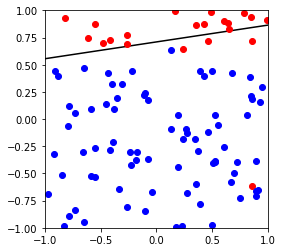
cannot converged in 101 iterations 
weight vector: [-0.4        -0.08723007  0.56359207]

Pocket

X,y,w,b = generate_non_separable_data(100)
p = Pocket()
p.fit(X,y)

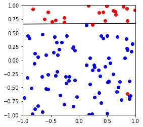
cannot converged in 101 iterations 
weight vector: [-0.4        -0.00380026  0.60356631]