https://pytorch.org/tutorials/beginner/deep_learning_60min_blitz.html
官方推荐的一篇教程
Tensors
#Construct a 5x3 matrix, uninitialized:
x = torch.empty(5, 3)

#Construct a randomly initialized matrix:
x = torch.rand(5, 3)

# Construct a matrix filled zeros and of dtype long:
x = torch.zeros(5, 3, dtype=torch.long)

# Construct a tensor directly from data:
x = torch.tensor([5.5, 3])

# create a tensor based on an existing tensor. These methods will reuse properties of the input tensor, e.g. dtype, unless new values are provided by user
x = x.new_ones(5, 3, dtype=torch.double)      # new_* methods take in sizes
print(x)
x = torch.randn_like(x, dtype=torch.float)    # override dtype!    #沿用了x已有的属性,只是修改dtype
print(x)                                      # result has the same size
tensor操作的语法有很多写法,以加法为例
#1
x = x.new_ones(5, 3, dtype=torch.double)
y = torch.rand(5, 3)
print(x + y)

#2
print(torch.add(x, y))

#3
result = torch.empty(5, 3)
torch.add(x, y, out=result)
print(result)

##注意以_做后缀的方法,都会改变原始的变量
#4 Any operation that mutates a tensor in-place is post-fixed with an _. For example: x.copy_(y), x.t_(), will change x.
# adds x to y
y.add_(x)
print(y)
改变tensor的size,使用torch.view:
x = torch.randn(4, 4)
y = x.view(16)
z = x.view(-1, 8)  # the size -1 is inferred from other dimensions
print(x.size(), y.size(), z.size())

输出如下:
torch.Size([4, 4]) torch.Size([16]) torch.Size([2, 8])
numpy array和torch tensor的相互转换
- torch tensor转换为numpy array
a = torch.ones(5)
print(a)
输出tensor([1., 1., 1., 1., 1.])

#torch tensor--->numpy array
b = a.numpy()
print(b)
输出[1. 1. 1. 1. 1.]


#注意!:a,b同时发生了变化
a.add_(1)
print(a)
print(b)
输出tensor([2., 2., 2., 2., 2.])
   [2. 2. 2. 2. 2.]
- numpy array转换为torch tensor
a = np.ones(5)
b = torch.from_numpy(a)
np.add(a, 1, out=a)
所有的cpu上的tensor,除了chartensor,都支持和numpy之间的互相转换.
All the Tensors on the CPU except a CharTensor support converting to NumPy and back.
CUDA Tensors
Tensors can be moved onto any device using the .to method.
#let us run this cell only if CUDA is available
#We will use ``torch.device`` objects to move tensors in and out of GPU
if torch.cuda.is_available():
    device = torch.device("cuda")          # a CUDA device object
    y = torch.ones_like(x, device=device)  # directly create a tensor on GPU
    x = x.to(device)                       # or just use strings ``.to("cuda")``
    z = x + y
    print(z)
    print(z.to("cpu", torch.double))       # ``.to`` can also change dtype together!

--->
tensor([0.6635], device='cuda:0')
tensor([0.6635], dtype=torch.float64)
AUTOGRAD
The autograd package provides automatic differentiation for all operations on Tensors. It is a define-by-run framework, which means that your backprop is defined by how your code is run, and that every single iteration can be different.
Generally speaking, torch.autograd is an engine for computing vector-Jacobian product
.requires_grad属性设为true,则可以追踪tensor上的所有操作(比如加减乘除)
torch.Tensor is the central class of the package. If you set its attribute .requires_grad as True, it starts to track all operations on it. When you finish your computation you can call .backward() and have all the gradients computed automatically. The gradient for this tensor will be accumulated into .grad attribute.
autograd包实现自动的求解梯度.
神经网络
torch.nn包可以用来构建神经网络.
nn依赖autogard来不断地更新model中各层的参数. nn.Module包含layers,forward方法.
典型的神经网络的训练过程如下:
- 定义一个神经网络,含learnable parameters或者叫weights
- 对数据集的所有数据作为Input输入网络
- 计算loss
- 反向传播计算weights的梯度
- 更新weights,一个典型的简单规则:weight = weight - learning_rate * gradient
定义网络
import torch
import torch.nn as nn
import torch.nn.functional as F
class Net(nn.Module):
def __init__(self):
super(Net, self).__init__()
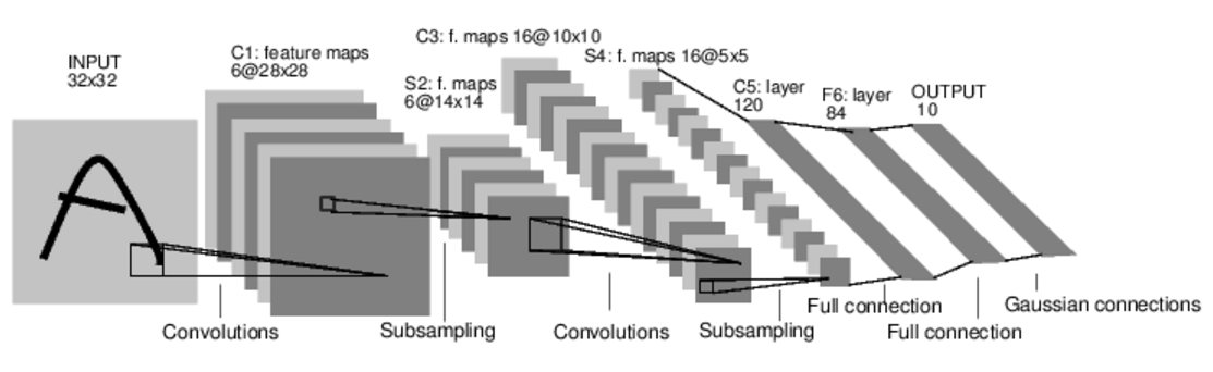
# 1 input image channel, 6 output channels, 5x5 square convolution
# kernel
self.conv1 = nn.Conv2d(1, 6, 5) #输入是1个矩阵,输出6个矩阵,filter是5*5矩阵.即卷积层1使用6个filter.
self.conv2 = nn.Conv2d(6, 16, 5) #输入是6个矩阵,输出16个矩阵,filter是5*5矩阵.即卷积层2使用16个filter.
# an affine operation: y = Wx + b
self.fc1 = nn.Linear(16 * 5 * 5, 120) #全连接层,fc=fullconnect 作用是分类
self.fc2 = nn.Linear(120, 84)
self.fc3 = nn.Linear(84, 10)
def forward(self, x):
# Max pooling over a (2, 2) window
x = F.max_pool2d(F.relu(self.conv1(x)), (2, 2))
# If the size is a square you can only specify a single number
x = F.max_pool2d(F.relu(self.conv2(x)), 2)
x = x.view(-1, self.num_flat_features(x))
x = F.relu(self.fc1(x))
x = F.relu(self.fc2(x))
x = self.fc3(x)
return x
def num_flat_features(self, x):
size = x.size()[1:] # all dimensions except the batch dimension
num_features = 1
for s in size:
num_features *= s
return num_features
net = Net()
print(net)
输出如下:
Net(
(conv1): Conv2d(1, 6, kernel_size=(5, 5), stride=(1, 1))
(conv2): Conv2d(6, 16, kernel_size=(5, 5), stride=(1, 1))
(fc1): Linear(in_features=400, out_features=120, bias=True)
(fc2): Linear(in_features=120, out_features=84, bias=True)
(fc3): Linear(in_features=84, out_features=10, bias=True)
)
你只需要定义forward函数,backward函数(即计算梯度的函数)是autograd包自动定义的.你可以在forward函数里使用任何tensor操作.
model的参数获取.
params = list(net.parameters())
print(len(params))
print(params[0].size())  # conv1's .weight

输出如下:
10
torch.Size([6, 1, 5, 5])
以MNIST识别为例,输入图像为3232.我们用一个随机的3232输入演示一下.
input = torch.randn(1, 1, 32, 32)
out = net(input)
print(out)

输出如下:
tensor([[ 0.0659, -0.0456,  0.1248, -0.1571, -0.0991, -0.0494,  0.0046, -0.0767,
         -0.0345,  0.1010]], grad_fn=<AddmmBackward>)


#清空所有的parameter的gradient buffer.用随机的梯度反向传播。
#Zero the gradient buffers of all parameters and backprops with random gradients:
net.zero_grad()
out.backward(torch.randn(1, 10))
回忆一下部分概念
- torch.Tensor - A multi-dimensional array with support for autograd operations like backward(). Also holds the gradient w.r.t. the tensor.
- nn.Module - Neural network module. Convenient way of encapsulating parameters, with helpers for moving them to GPU, exporting, loading, etc.
- nn.Parameter - A kind of Tensor, that is automatically registered as a parameter when assigned as an attribute to a Module.
- autograd.Function - Implements forward and backward definitions of an autograd operation. Every Tensor operation creates at least a single Function node that connects to functions that created a Tensor and encodes its history.
损失函数
nn package有好几种损失函数.以nn.MSELoss为例
output = net(input)
target = torch.randn(10)  # a dummy target, for example
target = target.view(1, -1)  # make it the same shape as output
criterion = nn.MSELoss()

loss = criterion(output, target)
print(loss)

输出
tensor(0.6918, grad_fn=<MseLossBackward>)
Now, if you follow loss in the backward direction, using its .grad_fn attribute, you will see a graph of computations that looks like this:
input -> conv2d -> relu -> maxpool2d -> conv2d -> relu -> maxpool2d
-> view -> linear -> relu -> linear -> relu -> linear
-> MSELoss
-> loss
print(loss.grad_fn)  # MSELoss
print(loss.grad_fn.next_functions[0][0])  # Linear
print(loss.grad_fn.next_functions[0][0].next_functions[0][0])  # ReLU
输出如下:
<MseLossBackward object at 0x7ff3406e1be0>
<AddmmBackward object at 0x7ff3406e1da0>
<AccumulateGrad object at 0x7ff3406e1da0>
反向传播
调用loss.backward()重新计算梯度
#首先清空现有的gradient buffer
net.zero_grad()     # zeroes the gradient buffers of all parameters

print('conv1.bias.grad before backward')
print(net.conv1.bias.grad)

loss.backward()

print('conv1.bias.grad after backward')
print(net.conv1.bias.grad)

输出如下:
conv1.bias.grad before backward
tensor([0., 0., 0., 0., 0., 0.])
conv1.bias.grad after backward
tensor([-0.0080,  0.0043, -0.0006,  0.0142, -0.0017, -0.0082])
更新权重
最常见的是使用随机梯度下降法更新权重:
weight = weight - learning_rate * gradient
简单实现如下
learning_rate = 0.01
for f in net.parameters():
    f.data.sub_(f.grad.data * learning_rate)
torch.optim包封装了各种各样的优化方法, SGD, Nesterov-SGD, Adam, RMSProp等等.
import torch.optim as optim

# create your optimizer
optimizer = optim.SGD(net.parameters(), lr=0.01)

# in your training loop:
optimizer.zero_grad()   # zero the gradient buffers
output = net(input)
loss = criterion(output, target)
loss.backward()
optimizer.step()    # Does the update