Linear regression
Files included in this exercise:
ex1.m - Octave/MATLAB script that steps you through the exercise
ex1 multi.m - Octave/MATLAB script for the later parts of the exercise
ex1data1.txt - Dataset for linear regression with one variable
ex1data2.txt - Dataset for linear regression with multiple variables
submit.m - Submission script that sends your solutions to our servers
[*] warmUpExercise.m - Simple example function in Octave/MATLAB
[*] plotData.m - Function to display the dataset
[*] computeCost.m - Function to compute the cost of linear regression
[*] gradientDescent.m - Function to run gradient descent
[*] computeCostMulti.m - Cost function for multiple variables
[*] gradientDescentMulti.m - Gradient descent for multiple variables
[*] featureNormalize.m - Function to normalize features
[*] normalEqn.m - Function to compute the normal equations
Linear regression with one variable
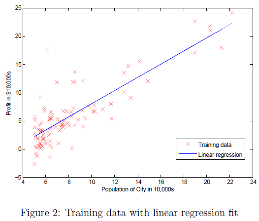
Problem: In this part of this exercise, you will implement linear regression with one variable to predict profi ts for a food truck. Suppose you are the CEO of a restaurant franchise and are considering different cities for opening a new outlet. The chain already has trucks in various cities and you have data for profits and populations from the cities. You would like to use this data to help you select which city to expand to next.
The main script:
%% Initialization clear ; close all; clc %% ==================== Part 1: Basic Function ==================== warmUpExercise()
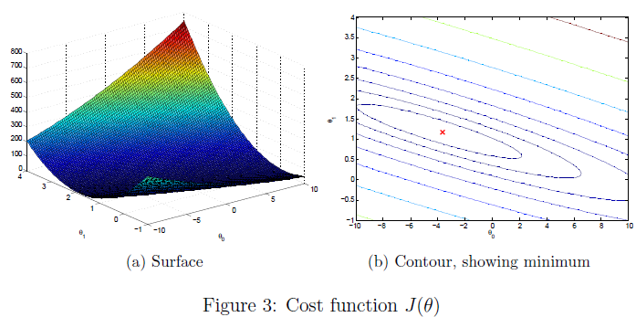
%% ======================= Part 2: Plotting ======================= fprintf('Plotting Data ... ') data = load('ex1data1.txt'); X = data(:, 1); y = data(:, 2); m = length(y); % number of training examples plotData(X, y); %% =================== Part 3: Cost and Gradient descent =================== X = [ones(m, 1), data(:,1)]; % Add a column of ones to x theta = zeros(2, 1); % initialize fitting parameters % Some gradient descent settings iterations = 1500; alpha = 0.01; % compute and display initial cost. The expected value is 32.07. J = computeCost(X, y, theta); % further testing of the cost function. The expected value is 54.24. J = computeCost(X, y, [-1 ; 2]); % run gradient descent theta = gradientDescent(X, y, theta, alpha, iterations); % Plot the linear fit hold on; % keep previous plot visible plot(X(:,2), X*theta, '-') legend('Training data', 'Linear regression') hold off % don't overlay any more plots on this figure % Predict values for population sizes of 35,000 and 70,000 predict1 = [1, 3.5] *theta; predict2 = [1, 7] * theta; %% ============= Part 4: Visualizing J(theta_0, theta_1) ============= fprintf('Visualizing J(theta_0, theta_1) ... ') % Grid over which we will calculate J theta0_vals = linspace(-10, 10, 100); theta1_vals = linspace(-1, 4, 100); % initialize J_vals to a matrix of 0's J_vals = zeros(length(theta0_vals), length(theta1_vals)); % Fill out J_vals for i = 1:length(theta0_vals) for j = 1:length(theta1_vals) t = [theta0_vals(i); theta1_vals(j)]; J_vals(i,j) = computeCost(X, y, t); end end % Because of the way meshgrids work in the surf command, we need to % transpose J_vals before calling surf, or else the axes will be flipped J_vals = J_vals'; % Surface plot figure; surf(theta0_vals, theta1_vals, J_vals) xlabel(' heta_0'); ylabel(' heta_1'); % Contour plot figure; % Plot J_vals as 15 contours spaced logarithmically between 0.01 and 100 contour(theta0_vals, theta1_vals, J_vals, logspace(-2, 3, 20)) xlabel(' heta_0'); ylabel(' heta_1'); hold on; plot(theta(1), theta(2), 'rx', 'MarkerSize', 10, 'LineWidth', 2);
warmUpExercise.m
function A = warmUpExercise()
A = eye(5);
end
plotData.m
function plotData(x, y)
figure;
plot(x,y,'rx', 'MarkerSize', 10);
ylabel('Profit in $10,000s');
xlabel('Population of City in 10,000s');
end
computeCost.m
function J = computeCost(X, y, theta)

m = length(y); % number of training examples
% You need to return the following variables correctly
J = 0;

temp1 = X*theta - y;
temp2 = temp1.*temp1;
J = sum(temp2(:))/(2*m);

end
gradientDescent.m
function [theta, J_history] = gradientDescent(X, y, theta, alpha, num_iters)

% Initialize some useful values
m = length(y); % number of training examples
J_history = zeros(num_iters, 1);

for iter = 1:num_iters
    temp = X'*(X*theta - y);
    theta = theta - alpha*temp/m;
    J_history(iter) = computeCost(X, y, theta);
end

end
Results:
Linear regression with multiple variables
Problem: Suppose you are selling your house and you want to know what a good market price would be. One way to do this is to first collect information on recent houses sold and make a model of housing prices.
The main script:
%% ================ Part 1: Feature Normalization ================
clear ; close all; clc
data = load('ex1data2.txt');
X = data(:, 1:2);
y = data(:, 3);
m = length(y);
% Scale features and set them to zero mean
[X mu sigma] = featureNormalize(X);
% Add intercept term to X
X = [ones(m, 1) X];
%% ================ Part 2: Gradient Descent ================
% Choose some alpha value
alpha = 0.01;
num_iters = 400;
% Init Theta and Run Gradient Descent
theta = zeros(3, 1);
[theta, J_history] = gradientDescentMulti(X, y, theta, alpha, num_iters);
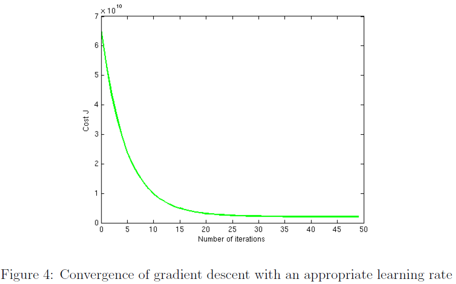
% Plot the convergence graph
figure;
plot(1:numel(J_history), J_history, '-b', 'LineWidth', 2);
xlabel('Number of iterations');
ylabel('Cost J');
% Estimate the price of a 1650 sq-ft, 3 br house
price = [1, 1650, 3]*theta;
%% ================ Part 3: Normal Equations ================
data = csvread('ex1data2.txt');
X = data(:, 1:2);
y = data(:, 3);
m = length(y);
% Add intercept term to X
X = [ones(m, 1) X];
% Calculate the parameters from the normal equation
theta = normalEqn(X, y);
% Estimate the price of a 1650 sq-ft, 3 br house. Should be same value as gradient descent.
price = [1, 1650, 3]*theta;
featureNormalize.m
function [X_norm, mu, sigma] = featureNormalize(X)
X_norm = X;
mu = zeros(1, size(X, 2));
sigma = zeros(1, size(X, 2));
mu = mean(X);
sigma = std(X);

for i = 1:length(mu)
  X_norm(:,i) = (X(:,i) - mu(1,i))/sigma(1,i);
end

end
gradientDescentMulti.m
function [theta, J_history] = gradientDescentMulti(X, y, theta, alpha, num_iters)

% Initialize some useful values
m = length(y); % number of training examples
J_history = zeros(num_iters, 1);

for iter = 1:num_iters
    temp = X'*(X*theta - y);
    theta = theta - alpha*temp/m;
    J_history(iter) = computeCostMulti(X, y, theta);

end

end
normalEqn.m
function [theta] = normalEqn(X, y)
theta = zeros(size(X, 2), 1);
theta = pinv(X'*X)*X'*y;
end
Results: