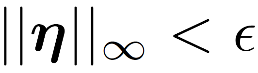
Early attempts at explaining this phenomenon focused on nonlinearity and overfitting. We argue instead that the primary cause of neural networks’ vulnerability to adversarial perturbation is their linear nature. Linear behavior in high-dimensional spaces is sufficient to cause adversarial examples. If we add a small perturbation on the original input x:

in which η is small enough, so that:
In a linear model, the output will increase by:
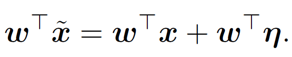
Because of the L infinite constraint, the maximum increase caused by the perturbation is to assign each element in η with absolute value Ɛ. The sign of η is same as the sign of ω, so that the weighted perturbation will increase the value of the equation.
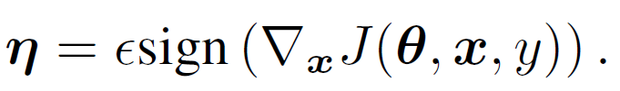
For a non-linear model, the weight cannot be derived directly. However, if we assume it is linear somehow, it can be calculated by taking derivative of the cost function. So using the same idear of adding perturbation on linear model. The adversarial perturbation is:
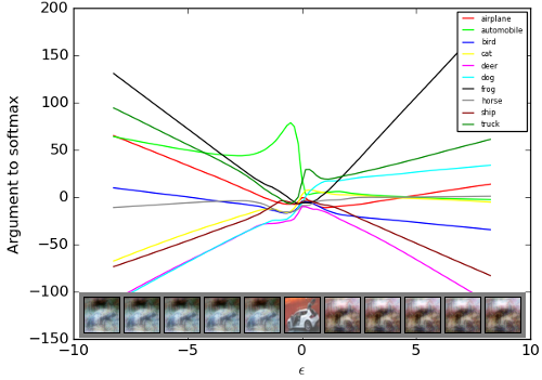
A very interesting finding: the relationship between input perturbation and output of neural network is very linear!
In many cases, a wide variety of models with different architectures trained on different subsets of the training data misclassify the same adversarial example. This suggests that adversarial examples expose fundamental blind spots in our training algorithms. On some datasets, such as ImageNet (Deng et al., 2009), the adversarial examples were so close to the original examples that the differences were indistinguishable to the human eye.
These results suggest that classifiers based on modern machine learning techniques, even those that obtain excellent performance on the test set, are not learning the true underlying concepts that determine the correct output label. Instead, these algorithms have built a Potemkin village that works well on naturally occuring data, but is exposed as a fake when one visits points in space that do not have high probability in the data distribution.
We mainly study on the relationship between parameters and outputs on Machine Learning courses, they are non-linear. How I make sense of it is that we can arbitrarily change parameters to generate a really non-linear output. However, when the parameters are fixed, the relationship between input and output is much linear than we expected. And in his reply on a forum, a graph is given to show how outputs of a model change as the perturbations change.
References:
Goodfellow, Ian J., et al. Explaining and Harnessing Adversarial Examples. Dec. 2014.
Goodfellow’s lecture on Adversarial Machine Learning:https://www.youtube.com/watch?v=CIfsB_EYsVI&t=1750s
Deep Learning Adversarial Examples – Clarifying Misconceptions: https://www.kdnuggets.com/2015/07/deep-learning-adversarial-examples-misconceptions.html
https://towardsdatascience.com/perhaps-the-simplest-introduction-of-adversarial-examples-ever-c0839a759b8d
https://towardsdatascience.com/know-your-adversary-understanding-adversarial-examples-part-1-2-63af4c2f5830