论文百度网盘链接:https://pan.baidu.com/s/1XWj1YInZCuKldRpYnZTttg
密码:u4lb
UCI数据可以在论文中给的一个URL中找到,如找不到也可联系QQ1551904915获取。
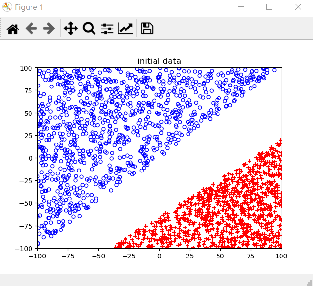
对类随机标签噪声下的二分类问题可以通过构造修正损失函数以及设置正负偏置两种方案解决。
流程:构造二维线性可分数据->UCI高维数据测试->构造二分线性不可分数据->UCI数据测试
import numpy as np
import matplotlib.pyplot as plt
import scipy.io as scio
from sklearn.preprocessing import StandardScaler
import math
from libsvm.svmutil import *
from sklearn.metrics import accuracy_score
from sklearn.model_selection import train_test_split


class LogisticRegression:
    def __init__(self, n_iter=200, eta=1e-3, tol=None,rho_positive = 0.2,rho_negative = 0.2):
        # 训练迭代次数
        self.n_iter = n_iter
        # 学习率
        self.eta = eta
        # 误差变化阈值
        self.tol = tol
        # 模型参数w(训练时初始化)
        self.w = None
        # 批量大小
        self.batch_size = 0.1
        self.rho_positive = rho_positive
        self.rho_negative = rho_negative

    def _z(self, X, w):
        return np.dot(X, w)

    def _sigmoid(self, z):
        return 1. / (1. + np.exp(-z))

    def _predict_proba(self, X, w):
        z = self._z(X, w)
        return self._sigmoid(z)

    # 标签噪声不存在时的梯度
    def _loss(self, y, y_proba):
        ret = 0
        for yi, ti in zip(y, y_proba):
            ret += np.log(1 + np.exp(- yi * ti))

        return ret + 1/2*np.dot(self.w,self.w)

    # 标签噪声不存在时的梯度
    def _gradient(self, X, y):
        ret = np.zeros_like(self.w)
        for xi,yi in zip(X,y):
            ti = np.dot(self.w.T,xi)
            ret += -yi*np.exp(-ti*yi)/(1+np.exp(-ti*yi)) * xi
        return ret + self.w

    # 存在标签噪声情况下的SGD
    def _gradient_descent_under_noise(self, w, X, y):

        # 若用户指定tol, 则启用早期停止法.
        if self.tol is not None:
            loss_old = np.inf

        self.loss_list = []
        self.w = w

        # 使用梯度下降至多迭代n_iter次, 更新w.
        for step_i in range(self.n_iter):
            # 预测所有点为1的概率
            y_proba = self._predict_proba(X, self.w)
            # 计算损失
            loss = self._loss_under_noise(y, y_proba)
            self.loss_list.append(loss)
            # print('%4i Loss: %s' % (step_i, loss))

            # 早期停止法
            if self.tol is not None:
                # 如果损失下降不足阈值, 则终止迭代.
                if loss_old - loss < self.tol:
                    break
                loss_old = loss

            index = np.arange(X.shape[0])
            np.random.shuffle(index)
            selected = index[:math.ceil(self.batch_size * X.shape[0])]
            # 计算梯度
            grad = self._gradient_under_noise(X[selected], y[selected])
            # 更新参数w
            self.w -= self.eta * grad

    def _gradient_descent(self, w, X, y):

        # 若用户指定tol, 则启用早期停止法.
        if self.tol is not None:
            loss_old = np.inf

        self.loss_list = []
        self.w = w

        # 使用梯度下降至多迭代n_iter次, 更新w.
        for step_i in range(self.n_iter):
            # 预测所有点为1的概率
            y_proba = self._predict_proba(X, self.w)
            # 计算损失
            loss = self._loss(y, y_proba)
            self.loss_list.append(loss)
            print('%4i Loss: %s' % (step_i, loss))
            if self.tol is not None:
                # 如果损失下降不足阈值, 则终止迭代.
                if loss_old - loss < self.tol:
                    break
                loss_old = loss

            index = np.arange(X.shape[0])
            np.random.shuffle(index)
            selected = index[:math.ceil(self.batch_size * X.shape[0])]
            # 计算梯度
            grad = self._gradient(X[selected], y[selected])
            # 更新参数w
            self.w -= self.eta * grad
    # 数据预处理
    def _preprocess_data_X(self, X):
        m, n = X.shape
        X_ = np.empty((m, n + 1))
        X_[:, 0] = 1
        X_[:, 1:] = X

        return X_

    def train(self, X_train, y_train):
        '''训练'''
        # 预处理X_train(添加x0=1)
        X_train = self._preprocess_data_X(X_train)
        _, n = X_train.shape
        self.w = np.random.random(n) * 0.05
        self._gradient_descent(self.w, X_train, y_train)


    def train_from_noise_data(self,X_train,y_train):
        X_train = self._preprocess_data_X(X_train)
        _,n = X_train.shape
        self.w = np.random.random(n) * 0.05
        self._gradient_descent_under_noise(self.w,X_train,y_train)

    #     计算在标签噪声下的损失
    def _loss_under_noise(self,y,y_proba):
        ret = 0
        for yi, ti in zip(y, y_proba):
            ret += (1-np.where(yi == 1,self.rho_negative,self.rho_positive)) * np.log(1 + np.exp(- yi * ti)) +
                   np.where(yi == 1,self.rho_positive,self.rho_negative) * np.log(1 + np.exp(yi * ti))

        return (ret + 1 / 2 * np.dot(self.w, self.w)) / (1 - self.rho_negative - self.rho_positive)
        # return (ret) / (1 - rho_negative - rho_positive)
    # 在标签噪声存在情况下的梯度
    def _gradient_under_noise(self,X,y):
        ret = np.zeros_like(self.w)
        for xi, yi in zip(X, y):
            ti = np.dot(self.w.T, xi)
            ret += (1-np.where(yi == 1,self.rho_negative,self.rho_positive)) * (-yi * np.exp(-ti * yi) / (1 + np.exp(-ti * yi)) * xi)
                + np.where(yi == 1,self.rho_positive,self.rho_negative) * (-yi * np.exp(ti * yi) / (1 + np.exp(ti * yi)) * xi)
        return (ret + self.w) / (1 - self.rho_negative - self.rho_positive)
        # return (ret) / (1 - rho_negative - rho_positive)

    def predict(self, X):

        X = self._preprocess_data_X(X)
        y_pred = self._predict_proba(X, self.w)
        return np.where(y_pred >= 0.5, 1, -1)

# 生成三角形区域的随机点集
def random_data(x1,y1,x2,y2,x3,y3):
    x1, y1 = x1, y1
    x3, y3 = x3, y3
    x2, y2 = x2, y2
    sample_size = 1000
    theta = np.arange(0, 1, 0.001)
    rnd1 = np.random.random(size=sample_size)
    rnd2 = np.random.random(size=sample_size)
    rnd2 = np.sqrt(rnd2)
    x = rnd2 * (rnd1 * x1 + (1 - rnd1) * x2) + (1 - rnd2) * x3
    y = rnd2 * (rnd1 * y1 + (1 - rnd1) * y2) + (1 - rnd2) * y3
    return x,y

def method_1_on_synthetic_data():
    x_positive, y_positive = random_data(-100, -100, -100, 100, 100, 100)
    x_negative, y_negative = random_data(-40, -100, 100, 20, 100, -100)
    x_data = np.concatenate([x_positive, x_negative])
    y_data = np.concatenate([y_positive, y_negative])
    label = np.concatenate([np.ones_like(x_positive), np.ones_like(x_negative) * (-1)])

    # view data from true distribution
    plt.scatter(x_data[label == 1], y_data[label == 1], c='', edgecolors='b', facecolor='none', marker='o', s=25,
                linewidths=1)
    plt.scatter(x_data[label == -1], y_data[label == -1], c='r', marker='+')
    plt.axis([-100, 100, -100, 100])
    plt.title('initial data')
    plt.show()

    print('=' * 10 + '在正确数据下的logistic预测' + '=' * 10)
    # view regression result from data without noise
    reg = LogisticRegression(n_iter=100, eta=0.0001, tol=1e-5)


    # 划分训练集以及测试集
    X_train, X_test, y_train, y_test = train_test_split(np.column_stack([x_data, y_data]), label, test_size=0.5)
    reg.train(X_train, y_train)

    plt.plot(reg.loss_list)
    plt.title('train loss with SGD')
    plt.show()

    y_pred = reg.predict(X_test)
    accuracy_rate = accuracy_score(y_test, y_pred)
    print('测试集上的训练准确度:', accuracy_rate)
    theta = reg.w
    print('theta参数为:', theta)
    print('分割函数:0={0}+({1})*x1+({2})*x2'.format(np.round(theta[0], 3), np.round(theta[1], 3), np.round(theta[2], 3)))

    rho_positive_list = [0.2,0.3,0.4]
    rho_negative_list = [0.2,0.1,0.4]
    print('=' * 10 + '在类标签噪声条件下的logistic预测' + '=' * 10)
    for index in range(3):
        mask_1 = np.random.uniform(0, 1, size=1000) < rho_positive_list[index]
        mask_2 = np.random.uniform(0, 1, size=1000) < rho_negative_list[index]

        label_dirty = np.concatenate([np.where(mask_1, -1, 1), np.where(mask_2, 1, -1)])

        # view regression result from data with noise
        plt.scatter(x_data[label_dirty == 1], y_data[label_dirty == 1], c='', edgecolors='b', facecolor='none', marker='o',
                    s=25,
                    linewidths=1)
        plt.scatter(x_data[label_dirty == -1], y_data[label_dirty == -1], c='r', marker='+')
        plt.axis([-100, 100, -100, 100])
        plt.title('dirty data with rho_positive = {0} and rho_negative = {1}'.format(rho_positive_list[index],rho_negative_list[index]))
        plt.show()


        reg = LogisticRegression(n_iter=1000, eta=0.00001, tol=1e-5, rho_positive=rho_positive_list[index], rho_negative=rho_negative_list[index])
        # 划分训练集以及测试集
        X_train = np.column_stack([x_data, y_data])
        reg.train_from_noise_data(X_train, label_dirty)

        y_pred = reg.predict(X_train)

        plt.scatter(x_data[y_pred == 1], y_data[y_pred == 1], c='', edgecolors='b', facecolor='none', marker='o', s=25,linewidths=1)
        plt.scatter(x_data[y_pred == -1], y_data[y_pred == -1], c='r', marker='+')
        plt.axis([-100, 100, -100, 100])
        plt.title('dirty data with rho_positive = {0} and rho_negative = {1}'.format(rho_positive_list[index], rho_negative_list[index]))
        plt.show()

        y_pred_under_noise = reg.predict(X_train)
        accuracy_rate = accuracy_score(label, y_pred_under_noise)
        print('rho_positive:{0} rho_negative:{1} accuracy:{2}'.format(rho_positive_list[index],rho_negative_list[index],accuracy_rate))
    print('='*20)

# 模拟模块
def train_mode(data,rho_negative,rho_positive,index):
    Xdata = data['x'][0][0]
    label = data['t'][0][0]
    sampleCapacity,_ = Xdata.shape
    dirty_label = np.zeros_like(label)
    # 构造噪声数据
    for i in range(sampleCapacity):
        if label[i] == 1:
            dirty_label[i] = np.where(np.random.uniform(0,1) < rho_positive,-1,1)
        else:
            dirty_label[i] = np.where(np.random.uniform(0,1) < rho_positive,1,-1)
    eta_list = [0.008,0.002,0.009]
    model = LogisticRegression(n_iter=1000, eta=eta_list[index], tol=1e-5, rho_positive=rho_positive, rho_negative=rho_negative)
    index = np.arange(sampleCapacity)
    np.random.shuffle(index)
    accuracy_rate = 0
    # 3折交叉验证
    for i in range(1, 4):
        # 构造索引集,将其中五分之一大小的一段作为测试集
        selected = np.array([False] * sampleCapacity)
        selected[int((i - 1) * sampleCapacity / 3):int(i * sampleCapacity / 3)] = True
        X_test = Xdata[index[selected]]
        X_train = Xdata[index[~selected]]
        # 对属性数据进行标准化,消除量纲以及数量级造成的差距
        ss = StandardScaler()
        ss.fit(X_train)
        X_train_std = ss.transform(X_train)
        X_test_std = ss.transform(X_test)
        y_train = dirty_label[index[~selected]]
        true_test_label = label[index[selected]]
        model.train_from_noise_data(X_train_std,y_train)
        pred = model.predict(X_test_std)
        accuracy_rate += accuracy_score(true_test_label,pred)

    print("rho_positive={0}  rho_negative={1} accuracy:{2}".format(rho_positive,rho_negative,round(accuracy_rate / 3,4)))

def train_mode_2(data,rho_negative,rho_positive,index):
    Xdata = data['x'][0][0]
    label = data['t'][0][0]
    label[label == -1] = 0
    sampleCapacity, _ = Xdata.shape
    dirty_label = np.zeros_like(label)
    # 构造噪声数据
    for i in range(sampleCapacity):
        if label[i] == 1:
            dirty_label[i] = np.where(np.random.uniform(0, 1) < rho_positive, 0, 1)
        else:
            dirty_label[i] = np.where(np.random.uniform(0, 1) < rho_positive, 1, 0)
    index = np.arange(sampleCapacity)
    np.random.shuffle(index)
    # 3折交叉验证
    for i in range(1, 4):
        # 构造索引集,将其中五分之一大小的一段作为测试集
        selected = np.array([False] * sampleCapacity)
        selected[int((i - 1) * sampleCapacity / 3):int(i * sampleCapacity / 3)] = True
        X_test = Xdata[index[selected]]
        X_train = Xdata[index[~selected]]
        # 对属性数据进行标准化,消除量纲以及数量级造成的差距
        ss = StandardScaler()
        ss.fit(X_train)
        X_train_std = ss.transform(X_train)
        X_test_std = ss.transform(X_test)
        y_train = dirty_label[index[~selected]]
        true_test_label = label[index[selected]]
        alpha = (1 - rho_positive + rho_negative) / 2
        model = svm_train(y_train.reshape(y_train.shape[0],),X_train_std,'-s 0 -t 2 -c 0.01 -w0 {0} -w1 {1}'.format(alpha,1 - alpha))
        svm_predict(true_test_label,X_test_std,model)


# logistic test on UCI benchmark
def method_1_on_UCI_benchmark():
    rho_positive_list = [0.2,0.3,0.4]
    rho_negative_list = [0.2,0.1,0.4]
    # 加载数据集
    benchmarks = scio.loadmat("benchmarks.mat")
    breastCancer = benchmarks['breast_cancer']
    diabetis = benchmarks['diabetis']
    thyroid = benchmarks['thyroid']
    german = benchmarks['german']
    heart = benchmarks['heart']
    image = benchmarks['image']

    print("test on breastCancer:")
    for i in range(3):
        train_mode(data=breastCancer,rho_negative=rho_negative_list[i],rho_positive=rho_positive_list[i],index = i)
    print("test on diabetis:")
    for i in range(3):
        train_mode(data=diabetis, rho_negative=rho_negative_list[i], rho_positive=rho_positive_list[i], index=i)
    print("test on thyroid:")
    for i in range(3):
        train_mode(data=thyroid, rho_negative=rho_negative_list[i], rho_positive=rho_positive_list[i], index=i)
    print("test on german:")
    for i in range(3):
        train_mode(data=german, rho_negative=rho_negative_list[i], rho_positive=rho_positive_list[i], index=i)
    print("test on heart:")
    for i in range(3):
        train_mode(data=heart, rho_negative=rho_negative_list[i], rho_positive=rho_positive_list[i], index=i)
    print("test on image:")
    for i in range(3):
        train_mode(data=image, rho_negative=rho_negative_list[i], rho_positive=rho_positive_list[i], index=i)
# C-SVM test on banana data
def method_2_on_banana_data():
    benchmarks = scio.loadmat("benchmarks.mat")
    banana = benchmarks['banana']
    y_data = banana['t'][0][0].reshape(banana['t'][0][0].shape[0], )
    y_data[y_data == -1] = 0
    x_data = banana['x'][0][0]
    plt.scatter(x_data[y_data == 1, 0], x_data[y_data == 1, 1], c='', edgecolors='b', facecolor='none',
                marker='o', s=25,
                linewidths=1)
    plt.scatter(x_data[y_data == 0, 0], x_data[y_data == 0, 1], c='r', marker='+')
    plt.title('initial image')
    plt.plot()
    plt.show()

    rho_positive_list = [0.2, 0.3, 0.4]
    rho_negative_list = [0.2, 0.1, 0.4]
    print('=' * 10 + '在类标签噪声条件下的C-SVM对香蕉数据的预测' + '=' * 10)
    for index in range(3):
        label_dirty = np.zeros_like(y_data)
        for i in range(label_dirty.shape[0]):
            if y_data[i] == 1:
                label_dirty[i] = np.where(np.random.uniform(0,1) < rho_positive_list[index],0,1)
            else:
                label_dirty[i] = np.where(np.random.uniform(0, 1) < rho_negative_list[index], 1, 0)

        # view regression result from data with noise
        plt.scatter(x_data[label_dirty == 1,0],
                    x_data[label_dirty == 1,1],
                    c='',
                    edgecolors='b',
                    facecolor='none',
                    marker='o',
                    s=25,
                    linewidths=1)
        plt.scatter(x_data[label_dirty == 0,0], x_data[label_dirty == 0,1], c='r', marker='+')
        plt.title('dirty data with rho_positive = {0} and rho_negative = {1}'.format(rho_positive_list[index],
                                                                                     rho_negative_list[index]))
        plt.show()

        # 划分训练集以及测试集
        X_train = np.column_stack([x_data, y_data])
        alpha = (1 - rho_positive_list[index] + rho_negative_list[index]) / 2
        model = svm_train(label_dirty,X_train,'-s 0 -t 2 -c 0.05 -w0 {0} -w1 {1}'.format(alpha,1 - alpha))
        # 在真实数据上进心预测
        y_pred = svm_predict(y_data,X_train,model)[0]
        y_pred = np.array(y_pred).astype('int64')
        # 绘制出预测之后的图像
        plt.scatter(x_data[y_pred == 1,0], x_data[y_pred == 1,1], c='', edgecolors='b', facecolor='none', marker='o', s=25,
                    linewidths=1)
        plt.scatter(x_data[y_pred == 0,0], x_data[y_pred == 0,1], c='r', marker='+')
        plt.title('dirty data with rho_positive = {0} and rho_negative = {1}'.format(rho_positive_list[index],
                                                                                     rho_negative_list[index]))
        plt.show()


    print('=' * 20)

def method_2_on_UCI_data():
    rho_positive_list = [0.2, 0.3, 0.4]
    rho_negative_list = [0.2, 0.1, 0.4]
    benchmarks = scio.loadmat("benchmarks.mat")
    breastCancer = benchmarks['breast_cancer']
    diabetis = benchmarks['diabetis']
    thyroid = benchmarks['thyroid']
    german = benchmarks['german']
    heart = benchmarks['heart']
    image = benchmarks['image']

    print('='*20+"test on breastCancer:"+'='*20)
    for i in range(3):
        train_mode_2(data=breastCancer, rho_negative=rho_negative_list[i], rho_positive=rho_positive_list[i], index=i)
    print('='*20+"test on diabetis:"+'='*20)
    for i in range(3):
        train_mode_2(data=diabetis, rho_negative=rho_negative_list[i], rho_positive=rho_positive_list[i], index=i)
    print('='*20+"test on thyroid:"+'='*20)
    for i in range(3):
        train_mode_2(data=thyroid, rho_negative=rho_negative_list[i], rho_positive=rho_positive_list[i], index=i)
    print('='*20+"test on german:"+'='*20)
    for i in range(3):
        train_mode_2(data=german, rho_negative=rho_negative_list[i], rho_positive=rho_positive_list[i], index=i)
    print('='*20+"test on heart:"+'='*20)
    for i in range(3):
        train_mode_2(data=heart, rho_negative=rho_negative_list[i], rho_positive=rho_positive_list[i], index=i)
    print('='*20+"test on image:"+'='*20)
    for i in range(3):
        train_mode_2(data=image, rho_negative=rho_negative_list[i], rho_positive=rho_positive_list[i], index=i)

if __name__ == '__main__':
    # 方法一在问题一的人造数据上进行测试
    method_1_on_synthetic_data()
    # 方法一在UCI数据上进行测试
    method_1_on_UCI_benchmark()
    # 方法二在香蕉数据上的可视化展示
    method_2_on_banana_data()
    # 方法二在UCI数据上进行测试
    method_2_on_UCI_data()
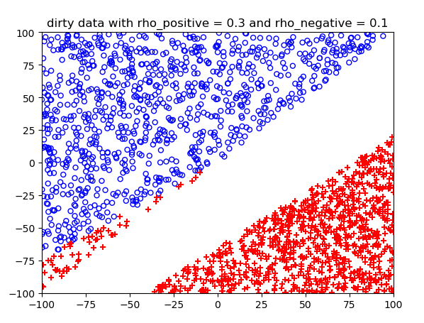
二分线性可分:
原数据:
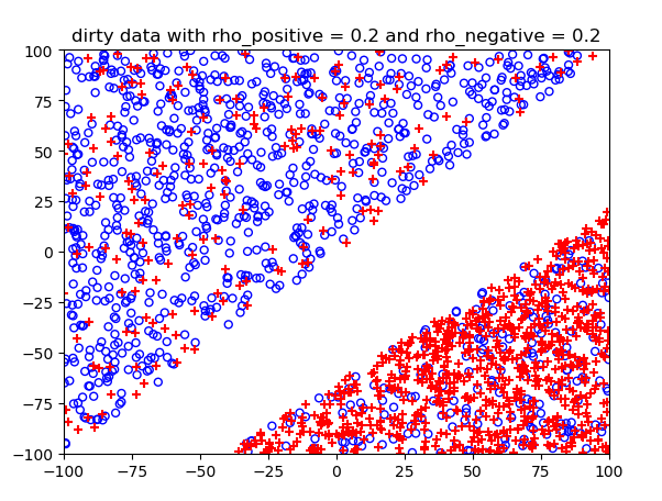
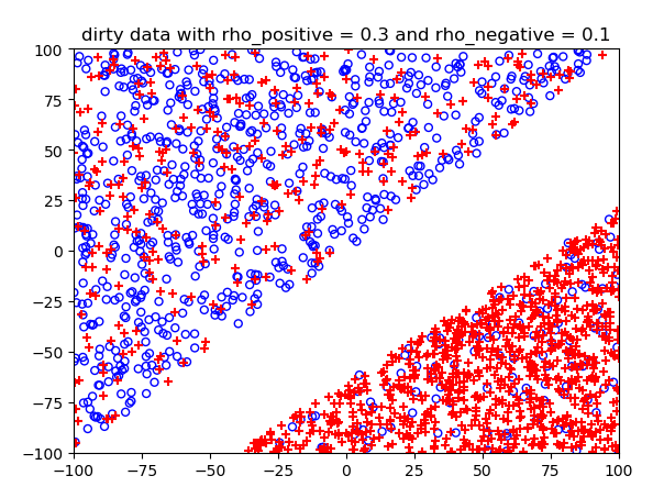
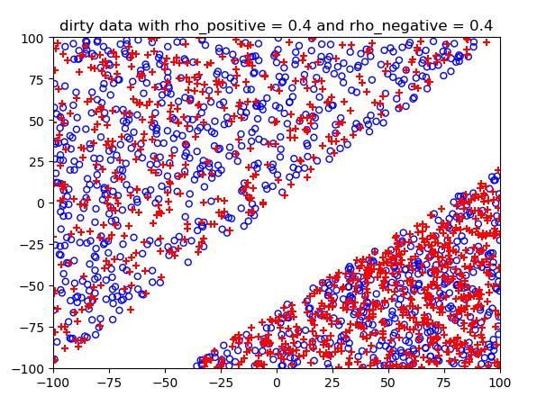
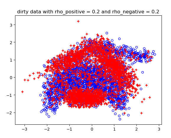
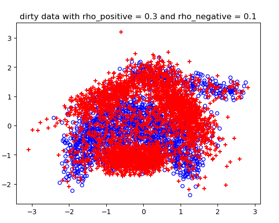
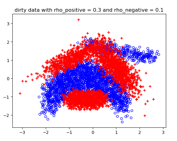
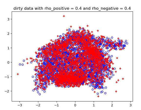
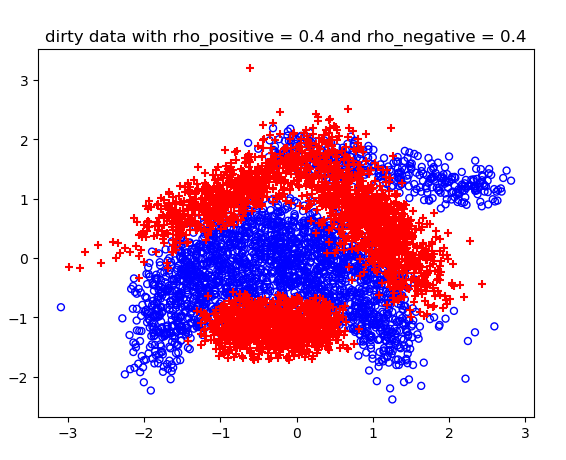
噪声概率不同情况下的结果:
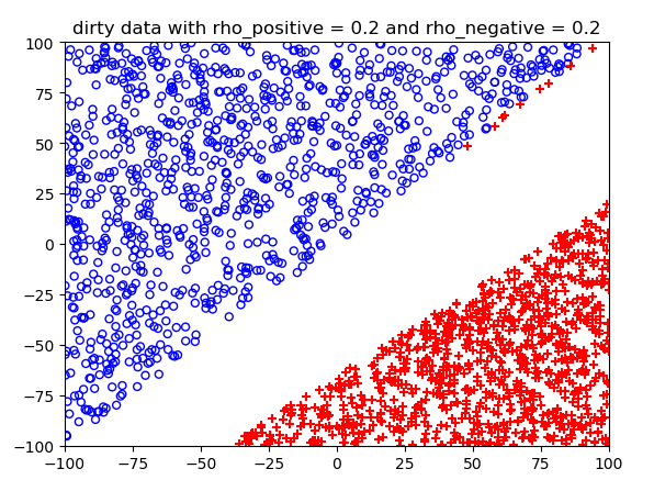
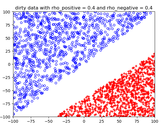
测试结果:
==========在正确数据下的logistic预测==========
   0 Loss: 655.0571765768963
   1 Loss: 523.6231639912271
   2 Loss: 508.3195448331075
   3 Loss: 506.8197572187573
   4 Loss: 506.8141896877468
   5 Loss: 506.68658996045286
   6 Loss: 507.0420107165859
测试集上的训练准确度: 0.993
theta参数为: [ 0.00242018 -0.16241579  0.15456798]
分割函数:0=0.002+(-0.162)*x1+(0.155)*x2
==========在类标签噪声条件下的logistic预测==========
rho_positive:0.2 rho_negative:0.2 accuracy:0.9955
rho_positive:0.3 rho_negative:0.1 accuracy:0.97
rho_positive:0.4 rho_negative:0.4 accuracy:1.0
====================
test on breastCancer:
rho_positive=0.2  rho_negative=0.2 accuracy:0.6314
rho_positive=0.3  rho_negative=0.1 accuracy:0.5319
rho_positive=0.4  rho_negative=0.4 accuracy:0.6239
test on diabetis:
rho_positive=0.2  rho_negative=0.2 accuracy:0.7474
rho_positive=0.3  rho_negative=0.1 accuracy:0.6654
rho_positive=0.4  rho_negative=0.4 accuracy:0.6107
test on thyroid:
rho_positive=0.2  rho_negative=0.2 accuracy:0.8184
rho_positive=0.3  rho_negative=0.1 accuracy:0.4797
rho_positive=0.4  rho_negative=0.4 accuracy:0.5445
test on german:
rho_positive=0.2  rho_negative=0.2 accuracy:0.696
rho_positive=0.3  rho_negative=0.1 accuracy:0.5609
rho_positive=0.4  rho_negative=0.4 accuracy:0.507
test on heart:
rho_positive=0.2  rho_negative=0.2 accuracy:0.8
rho_positive=0.3  rho_negative=0.1 accuracy:0.7667
rho_positive=0.4  rho_negative=0.4 accuracy:0.6704
test on image:
rho_positive=0.2  rho_negative=0.2 accuracy:0.7171
rho_positive=0.3  rho_negative=0.1 accuracy:0.6961
rho_positive=0.4  rho_negative=0.4 accuracy:0.6424
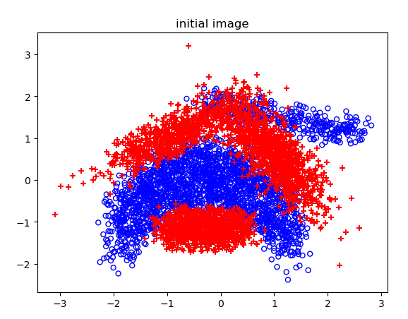
二维线性不可分:
原图:
不同噪声情况下的分类结果:

高维的C-SVM结果比较长,不展示了。