在回归问题中,我们的目标是预测连续值的输出,如价格或概率。 我们采用了经典的Auto MPG数据集,并建立了一个模型来预测20世纪70年代末和80年代初汽车的燃油效率。 为此,我们将为该模型提供该时段内许多汽车的描述。 此描述包括以下属性:气缸,排量,马力和重量。
1.Auto MPG数据集
获取数据
dataset_path = keras.utils.get_file('auto-mpg.data',
                                   'https://archive.ics.uci.edu/ml/machine-learning-databases/auto-mpg/auto-mpg.data')

print(dataset_path)
Downloading data from https://archive.ics.uci.edu/ml/machine-learning-databases/auto-mpg/auto-mpg.data
32768/30286 [================================] - 1s 25us/step
/home/czy/.keras/datasets/auto-mpg.data
使用pandas读取数据
column_names = ['MPG','Cylinders','Displacement','Horsepower','Weight',
                'Acceleration', 'Model Year', 'Origin']
raw_dataset = pd.read_csv(dataset_path, names=column_names,
                         na_values='?', comment='	',
                         sep=' ', skipinitialspace=True)
dataset = raw_dataset.copy()
dataset.tail()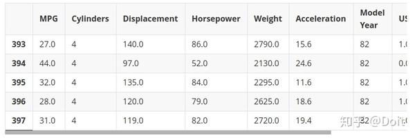
2.数据预处理
清洗数据
print(dataset.isna().sum())
dataset = dataset.dropna()
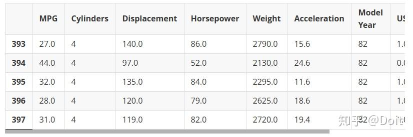
origin = dataset.pop('Origin')
dataset['USA'] = (origin == 1)*1.0
dataset['Europe'] = (origin == 2)*1.0
dataset['Japan'] = (origin == 3)*1.0
dataset.tail()
MPG 0
Cylinders 0
Displacement 0
Horsepower 6
Weight 0
Acceleration 0
Model Year 0
Origin 0
dtype: int64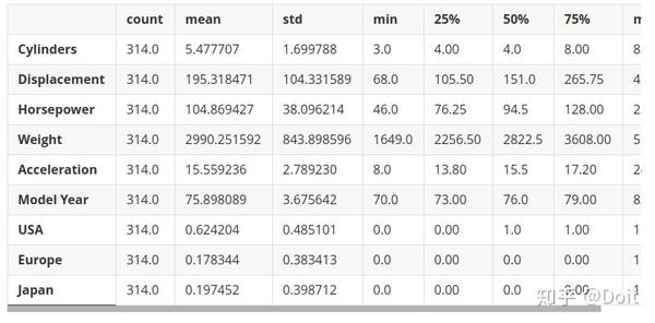
划分训练集和测试集
train_dataset = dataset.sample(frac=0.8,random_state=0)
test_dataset = dataset.drop(train_dataset.index)
检测数据
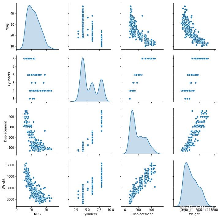
观察训练集中几对列的联合分布。
sns.pairplot(train_dataset[["MPG", "Cylinders", "Displacement", "Weight"]], diag_kind="kde")
<seaborn.axisgrid.PairGrid at 0x7f934072fe10>

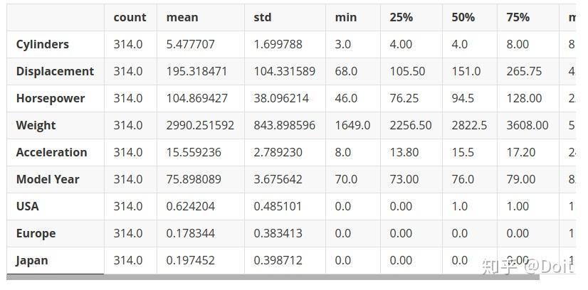
整体统计数据:
train_stats = train_dataset.describe()
train_stats.pop("MPG")
train_stats = train_stats.transpose()
train_stats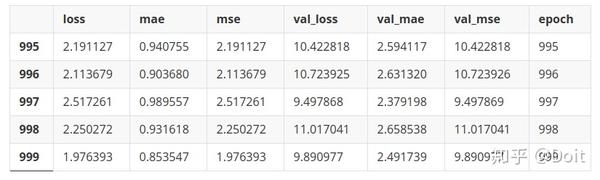
取出标签
train_labels = train_dataset.pop('MPG')
test_labels = test_dataset.pop('MPG')
标准化数据
最好使用不同比例和范围的特征进行标准化。 虽然模型可能在没有特征归一化的情况下收敛,但它使训练更加困难,并且它使得结果模型依赖于输入中使用的单位的选择。
def norm(x):
    return (x - train_stats['mean']) / train_stats['std']
normed_train_data = norm(train_dataset)
normed_test_data = norm(test_dataset)
3.构建模型
def build_model():
    model = keras.Sequential([
        layers.Dense(64, activation='relu', input_shape=[len(train_dataset.keys())]),
        layers.Dense(64, activation='relu'),
        layers.Dense(1)
    ])

    optimizer = tf.keras.optimizers.RMSprop(0.001)
    model.compile(loss='mse',
                 optimizer=optimizer,
                 metrics=['mae', 'mse'])
    return model
model = build_model()
model.summary()
Model: "sequential"
_________________________________________________________________
Layer (type)                 Output Shape              Param #
=================================================================
dense (Dense)                (None, 64)                640
_________________________________________________________________
dense_1 (Dense)              (None, 64)                4160
_________________________________________________________________
dense_2 (Dense)              (None, 1)                 65
=================================================================
Total params: 4,865
Trainable params: 4,865
Non-trainable params: 0
_________________________________________________________________
example_batch = normed_train_data[:10]
example_result = model.predict(example_batch)
example_result
array([[0.18062565],
       [0.1714489 ],
       [0.22555563],
       [0.29366603],
       [0.69764495],
       [0.08851457],
       [0.6851174 ],
       [0.32245407],
       [0.02959149],
       [0.38945067]], dtype=float32)
4.训练模型
class PrintDot(keras.callbacks.Callback):
def on_epoch_end(self, epoch, logs):
if epoch % 100 == 0: print('')
print('.', end='')
EPOCHS = 1000
history = model.fit(
normed_train_data, train_labels,
epochs=EPOCHS, validation_split = 0.2, verbose=0,
callbacks=[PrintDot()])
....................................................................................................
....................................................................................................
....................................................................................................
....................................................................................................
....................................................................................................
....................................................................................................
....................................................................................................
....................................................................................................
....................................................................................................
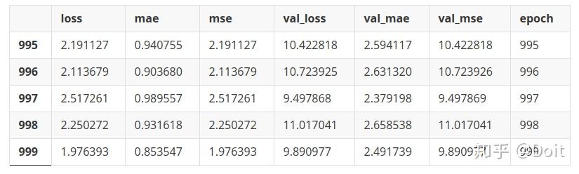
....................................................................................................查看训练记录
hist = pd.DataFrame(history.history)
hist['epoch'] = history.epoch
hist.tail()
loss mae mse val_loss val_mae val_mse epoch 995 2.191127 0.940755 2.191127 10.422818 2.594117 10.422818 995 996 2.113679 0.903680 2.113679 10.723925 2.631320 10.723926 996 997 2.517261 0.989557 2.517261 9.497868 2.379198 9.497869 997 998 2.250272 0.931618 2.250272 11.017041 2.658538 11.017041 998 999 1.976393 0.853547 1.976393 9.890977 2.491739 9.890977 999
def plot_history(history):
hist = pd.DataFrame(history.history)
hist['epoch'] = history.epoch
plt.figure()
plt.xlabel('Epoch')
plt.ylabel('Mean Abs Error [MPG]')
plt.plot(hist['epoch'], hist['mae'],
label='Train Error')
plt.plot(hist['epoch'], hist['val_mae'],
label = 'Val Error')
plt.ylim([0,5])
plt.legend()
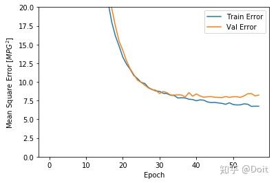
plt.figure()
plt.xlabel('Epoch')
plt.ylabel('Mean Square Error [$MPG^2$]')
plt.plot(hist['epoch'], hist['mse'],
label='Train Error')
plt.plot(hist['epoch'], hist['val_mse'],
label = 'Val Error')
plt.ylim([0,20])
plt.legend()
plt.show()
plot_history(history)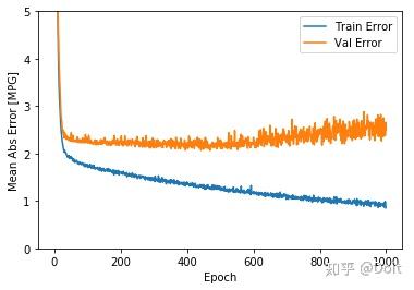

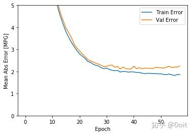
使用early stop
model = build_model()


early_stop = keras.callbacks.EarlyStopping(monitor='val_loss', patience=10)

history = model.fit(normed_train_data, train_labels, epochs=EPOCHS,
                    validation_split = 0.2, verbose=0, callbacks=[early_stop, PrintDot()])

plot_history(history)
..........................................................
测试
loss, mae, mse = model.evaluate(normed_test_data, test_labels, verbose=0)

print("Testing set Mean Abs Error: {:5.2f} MPG".format(mae))
Testing set Mean Abs Error:  1.85 MPG
5.预测
test_predictions = model.predict(normed_test_data).flatten()
plt.scatter(test_labels, test_predictions)
plt.xlabel('True Values [MPG]')
plt.ylabel('Predictions [MPG]')
plt.axis('equal')
plt.axis('square')
plt.xlim([0,plt.xlim()[1]])
plt.ylim([0,plt.ylim()[1]])
_ = plt.plot([-100, 100], [-100, 100])
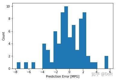
error = test_predictions - test_labels
plt.hist(error, bins = 25)
plt.xlabel("Prediction Error [MPG]")
_ = plt.ylabel("Count")