使用TensorFlow v2.0实现逻辑斯谛回归
此示例使用简单方法来更好地理解训练过程背后的所有机制
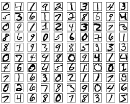
MNIST数据集概览
此示例使用MNIST手写数字。该数据集包含60,000个用于训练的样本和10,000个用于测试的样本。这些数字已经过尺寸标准化并位于图像中心,图像是固定大小(28x28像素),其值为0到255。
在此示例中,每个图像将转换为float32,归一化为[0,1],并展平为784个特征(28 * 28)的1维数组。
from __future__ import absolute_import,division,print_function

import tensorflow as tf
import numpy as np
# MNIST 数据集参数
num_classes = 10 # 数字0-9
num_features = 784 # 28*28

# 训练参数
learning_rate = 0.01
training_steps = 1000
batch_size = 256
display_step = 50
# 准备MNIST数据
from tensorflow.keras.datasets import mnist
(x_train, y_train),(x_test,y_test) = mnist.load_data()
# 转换为float32
x_train, x_test = np.array(x_train, np.float32), np.array(x_test, np.float32)
# 将图像平铺成784个特征的一维向量(28*28)
x_train, x_test = x_train.reshape([-1, num_features]), x_test.reshape([-1, num_features])
# 将像素值从[0,255]归一化为[0,1]
x_train,x_test = x_train / 255, x_test / 255
# 使用tf.data api 对数据随机分布和批处理
train_data = tf.data.Dataset.from_tensor_slices((x_train, y_train))
train_data = train_data.repeat().shuffle(5000).batch(batch_size).prefetch(1)
# 权值矩阵形状[784,10],28 * 28图像特征数和类别数目
W = tf.Variable(tf.ones([num_features, num_classes]), name="weight")
# 偏置形状[10], 类别数目
b = tf.Variable(tf.zeros([num_classes]), name="bias")

# 逻辑斯谛回归(Wx b)
def logistic_regression(x):
    #应用softmax将logits标准化为概率分布
    return tf.nn.softmax(tf.matmul(x,W)   b)

# 交叉熵损失函数
def cross_entropy(y_pred, y_true):
    # 将标签编码为一个独热编码向量
    y_true = tf.one_hot(y_true, depth=num_classes)
    # 压缩预测值以避免log(0)错误
    y_pred = tf.clip_by_value(y_pred, 1e-9, 1.)
    # 计算交叉熵
    return tf.reduce_mean(-tf.reduce_sum(y_true * tf.math.log(y_pred)))

# 准确率度量
def accuracy(y_pred, y_true):
    # 预测的类别是预测向量中最高分的索引(即argmax)
    correct_prediction = tf.equal(tf.argmax(y_pred, 1), tf.cast(y_true, tf.int64))
    return tf.reduce_mean(tf.cast(correct_prediction, tf.float32))

# 随机梯度下降优化器
optimizer = tf.optimizers.SGD(learning_rate)
# 优化过程
def run_optimization(x, y):
    #将计算封装在GradientTape中以实现自动微分
    with tf.GradientTape() as g:
        pred = logistic_regression(x)
        loss = cross_entropy(pred, y)

    # 计算梯度
    gradients = g.gradient(loss, [W, b])

    # 根据gradients更新 W 和 b
    optimizer.apply_gradients(zip(gradients, [W, b]))
# 针对给定训练步骤数开始训练
for step, (batch_x,batch_y) in enumerate(train_data.take(training_steps), 1):
    # 运行优化以更新W和b值
    run_optimization(batch_x, batch_y)

    if step % display_step == 0:
        pred = logistic_regression(batch_x)
        loss = cross_entropy(pred, batch_y)
        acc = accuracy(pred, batch_y)
        print("step: %i, loss: %f, accuracy: %f" % (step, loss, acc))
output:
step: 50, loss: 608.584717, accuracy: 0.824219
step: 100, loss: 828.206482, accuracy: 0.765625
step: 150, loss: 716.329407, accuracy: 0.746094
step: 200, loss: 584.887634, accuracy: 0.820312
step: 250, loss: 472.098114, accuracy: 0.871094
step: 300, loss: 621.834595, accuracy: 0.832031
step: 350, loss: 567.288818, accuracy: 0.714844
step: 400, loss: 489.062988, accuracy: 0.847656
step: 450, loss: 496.466675, accuracy: 0.843750
step: 500, loss: 465.342224, accuracy: 0.875000
step: 550, loss: 586.347168, accuracy: 0.855469
step: 600, loss: 95.233109, accuracy: 0.906250
step: 650, loss: 88.136490, accuracy: 0.910156
step: 700, loss: 67.170349, accuracy: 0.937500
step: 750, loss: 79.673691, accuracy: 0.921875
step: 800, loss: 112.844872, accuracy: 0.914062
step: 850, loss: 92.789581, accuracy: 0.894531
step: 900, loss: 80.116165, accuracy: 0.921875
step: 950, loss: 45.706650, accuracy: 0.925781
step: 1000, loss: 72.986969, accuracy: 0.925781
# 在验证集上测试模型
pred = logistic_regression(x_test)
print("Test Accuracy: %f" % accuracy(pred, y_test))
output:
Test Accuracy: 0.901100
# 可视化预测
import matplotlib.pyplot as plt

# 在验证集上中预测5张图片
n_images = 5
test_images = x_test[:n_images]
predictions = logistic_regression(test_images)

# 可视化图片和模型预测结果
for i in range(n_images):
    plt.imshow(np.reshape(test_images[i],[28,28]), cmap='gray')
    plt.show()
    print("Model prediction: %i" % np.argmax(predictions.numpy()[i]))
output:
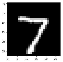
Model prediction: 7
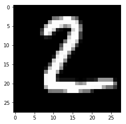
Model prediction: 2
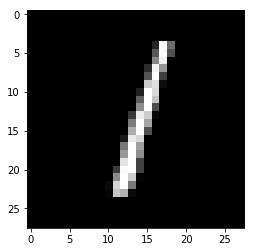
Model prediction: 1
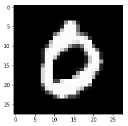
Model prediction: 0
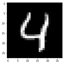
Model prediction: 4
欢迎关注磐创博客资源汇总站:
http://docs.panchuang.net/
欢迎关注PyTorch官方中文教程站:
http://pytorch.panchuang.net/