1.1.2 Building basic functions with numpy
1.1.2.2 numpy.exp, sigmoid, sigmoid gradient
import numpy as np

def sigmoid(x):
    s = 1/(1+np.exp(-x))
    return s

# 设sigmoid为s, s' = s*(1-s)
def sigmoid_derivative(x):
    s = 1/(1+np.exp(-x))
    ds = s*(1-s)
    return ds

plt.figure(1)  # 编号为1的figure
x = np.arange(-5, 5, 0.1)
y = sigmoid(x)
plt.subplot(211)  # 将子图划分为2行,1列,选中2行中的第1行
plt.plot(x, y)

y = sigmoid_derivative(x)
plt.subplot(212)  # 子图中2行中的第2行
plt.plot(x, y)
plt.show()
1.1.2.3 numpy.reshape(), numpy.shape
def image2vector(image):
    """
    Argument:
    image -- a numpy array of shape (length, height, depth)

    Returns:
    v -- a vector of shape (length*height*depth, 1)
    """

    v = image.reshape(image.shape[0] * image.shape[1] * image.shape[2], 1)

    return v
1.1.2.4 Normalizing rows
np.linalg.norm求对矩阵x按axis作向量内积
def normalizeRows(x):
    """
    Implement a function that normalizes each row of the matrix x (to have
    unit length).

    Argument:
    x -- A numpy matrix of shape (n, m)

    Returns:
    x -- The normalized (by row) numpy matrix. You are allowed to modify x.
    """
    # Compute x_norm as the norm 2 of x. Use np.linalg.norm(..., ord = 2,
    # axis = ..., keepdims = True)
    # linalg=linear+algebra.
    x_norm = np.linalg.norm(x, axis=1, keepdims=True)

    # Divide x by its norm.
    x = x/x_norm
    return x

x = np.array([
    [0, 3, 4],
    [1, 6, 4]
    ])
print("normalizeRows(x) = " + str(normalizeRows(x)))
1.1.2.5 Broadcasting and the softmax function
def softmax(x):
    x_exp = np.exp(x)
    s_sum = np.sum(x_exp, axis=1, keepdims=True)
    s = x_exp/s_sum
    return s
 来,敲黑板:
1.np.exp(x)对任何np.array的x都可以使用并且是对每个元素进行的求指数
2.sigmoid函数以及其导数
3.image2vector在深度学习中很常用
4.np.reshape应用很广泛。保持矩阵/向量的维度会消除大量的BUG。
5.numpy有很多高效的内建函数。
6.广播非常非常有用
1.1.2 Vectorization
import time

x1 = [9, 2, 5, 0, 0, 7, 5, 0, 0, 0, 9, 2, 5, 0, 0]
x2 = [9, 2, 2, 9, 0, 9, 2, 5, 0, 0, 9, 2, 5, 0, 0]

### CLASSIC DOT PRODUCT OF VECTORS IMPLEMENTATION ###
### 向量点乘(内积): a▪b = a^T*b (-|型)= a1b1+a2b2+......+anbn

tic = time.process_time()
dot = 0
for i in range(len(x1)):
    dot += x1[i]*x2[i]
toc = time.process_time()
print("dot = " + str(dot) + "
 ----- Computation time = " +
        str(1000*(toc - tic)) + "ms")

### CLASSIC OUTER PRODUCT IMPLEMENTATION ###
### 向量叉乘(外积): axb = a*b^T (|-型)

tic = time.process_time()
outer = np.zeros((len(x1), len(x2))) # we create a len(x1)*len(x2) matrix with
    # only zeros
for i in range(len(x1)):
    for j in range(len(x2)):
        outer[i, j] = x1[i] * x2[j]
toc = time.process_time()
print("outer = " + str(outer) + "
 ----- Computation time = " +
        str(1000*(toc - tic)) + "ms")

### CLASSIC ELEMENTWISE IMPLEMENTATION ###
### 向量元素依次相乘

tic = time.process_time()
mul = np.zeros(len(x1))
for i in range(len(x1)):
    mul[i] = x1[i] * x2[i]
toc = time.process_time()
print("elementwise multiplication = " + str(mul) +
        "
 ----- Computation time = " + str(1000*(toc - tic)) + "ms")

### CLASSIC GENERAL DOT PRODUCT IMPLEMENTATION ###
###

W = np.random.rand(3, len(x1)) # Random 3*len(x1) numpy array
tic = time.process_time()
gdot = np.zeros(W.shape[0])
for i in range(W.shape[0]):
    for j in range(len(x1)):  # W的每一行与x1相乘
        gdot[i] += W[i,j]*x1[j]
toc = time.process_time()
print("gdot = " + str(gdot) + "
 ----- Computation time = " +
        str(1000*(toc - tic)) + "ms")
输出:
dot = 278
 ----- Computation time = 0.00854900000035741ms
outer = [[81. 18. 18. 81.  0. 81. 18. 45.  0.  0. 81. 18. 45.  0.  0.]
 [18.  4.  4. 18.  0. 18.  4. 10.  0.  0. 18.  4. 10.  0.  0.]
 [45. 10. 10. 45.  0. 45. 10. 25.  0.  0. 45. 10. 25.  0.  0.]
 [ 0.  0.  0.  0.  0.  0.  0.  0.  0.  0.  0.  0.  0.  0.  0.]
 [ 0.  0.  0.  0.  0.  0.  0.  0.  0.  0.  0.  0.  0.  0.  0.]
 [63. 14. 14. 63.  0. 63. 14. 35.  0.  0. 63. 14. 35.  0.  0.]
 [45. 10. 10. 45.  0. 45. 10. 25.  0.  0. 45. 10. 25.  0.  0.]
 [ 0.  0.  0.  0.  0.  0.  0.  0.  0.  0.  0.  0.  0.  0.  0.]
 [ 0.  0.  0.  0.  0.  0.  0.  0.  0.  0.  0.  0.  0.  0.  0.]
 [ 0.  0.  0.  0.  0.  0.  0.  0.  0.  0.  0.  0.  0.  0.  0.]
 [81. 18. 18. 81.  0. 81. 18. 45.  0.  0. 81. 18. 45.  0.  0.]
 [18.  4.  4. 18.  0. 18.  4. 10.  0.  0. 18.  4. 10.  0.  0.]
 [45. 10. 10. 45.  0. 45. 10. 25.  0.  0. 45. 10. 25.  0.  0.]
 [ 0.  0.  0.  0.  0.  0.  0.  0.  0.  0.  0.  0.  0.  0.  0.]
 [ 0.  0.  0.  0.  0.  0.  0.  0.  0.  0.  0.  0.  0.  0.  0.]]
 ----- Computation time = 0.12781600000000282ms
elementwise multiplication = [81.  4. 10.  0.  0. 63. 10.  0.  0.  0. 81.  4. 25.  0.  0.]
 ----- Computation time = 0.018939999999911805ms
gdot = [21.88386459 17.22658932 13.05841111]
 ----- Computation time = 0.07001299999975785ms
numpy实现
import time
import numpy as np

x1 = [9, 2, 5, 0, 0, 7, 5, 0, 0, 0, 9, 2, 5, 0, 0]
x2 = [9, 2, 2, 9, 0, 9, 2, 5, 0, 0, 9, 2, 5, 0, 0]

### VECTORIZED DOT PRODUCT OF VECTORS ###
tic = time.process_time()
dot = np.dot(x1, x2)
toc = time.process_time()
print("dot = " + str(dot) + "
 ----- Computation time = " +
        str(1000*(toc - tic)) + "ms")

### VECTORIZED OUTER PRODUCT ###
tic = time.process_time()
outer = np.outer(x1, x2)
toc = time.process_time()
print("outer = " + str(outer) + "
 ----- Computation time = " +
        str(1000*(toc - tic)) + "ms")

### VECOTRIZED ELEMENTWISE MULTIPLICATION ###
tic = time.process_time()
mul = np.multiply(x1, x2)
toc = time.process_time()
print("elementwise multiplication = " + str(mul) +
        "
 ----- Computation time = " + str(1000*(toc - tic)) + "ms")

### VECOTRIZED GENERAL DOT PRODUCT ###
W = np.random.rand(3, len(x1))
tic = time.process_time()
gdot = np.dot(W, x1)
toc = time.process_time()
print("gdot = " + str(gdot) + "
 ----- Computation time = " +
        str(1000*(toc - tic)) + "ms")
输出:
dot = 278
 ----- Computation time = 0.17038700000027163ms
outer = [[81 18 18 81  0 81 18 45  0  0 81 18 45  0  0]
 [18  4  4 18  0 18  4 10  0  0 18  4 10  0  0]
 [45 10 10 45  0 45 10 25  0  0 45 10 25  0  0]
 [ 0  0  0  0  0  0  0  0  0  0  0  0  0  0  0]
 [ 0  0  0  0  0  0  0  0  0  0  0  0  0  0  0]
 [63 14 14 63  0 63 14 35  0  0 63 14 35  0  0]
 [45 10 10 45  0 45 10 25  0  0 45 10 25  0  0]
 [ 0  0  0  0  0  0  0  0  0  0  0  0  0  0  0]
 [ 0  0  0  0  0  0  0  0  0  0  0  0  0  0  0]
 [ 0  0  0  0  0  0  0  0  0  0  0  0  0  0  0]
 [81 18 18 81  0 81 18 45  0  0 81 18 45  0  0]
 [18  4  4 18  0 18  4 10  0  0 18  4 10  0  0]
 [45 10 10 45  0 45 10 25  0  0 45 10 25  0  0]
 [ 0  0  0  0  0  0  0  0  0  0  0  0  0  0  0]
 [ 0  0  0  0  0  0  0  0  0  0  0  0  0  0  0]]
 ----- Computation time = 0.1971060000003355ms
elementwise multiplication = [81  4 10  0  0 63 10  0  0  0 81  4 25  0  0]
 ----- Computation time = 0.06556499999987864ms
gdot = [19.3061823  18.29576413 24.1581206 ]
 ----- Computation time = 0.06616899999967174ms
As you may have noticed, the vectorized implementation is much cleaner and more efcient. For bigger vectors/matrices, the differences in running time become even bigger.
 这里意思是numpy的向量化实现更加简洁和高效,对于更庞大的向量和矩阵,运行效率会相差更多。
 然鹅我运行出来明明是numpy运行时间更多一丢丢。。。估计和我的环境有关系???
 那么先不管了,接着刚下面的。。。
1.1.3.1 Implement the L1 and L2 loss functions
那么L1就是个这: 
L2就是个这: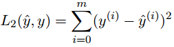
这里都是范式的概念,L1假设的是模型的参数取值满足拉普拉斯分布,L2假设的模型参数是满足高斯分布,所谓的范式其实就是加上对参数的约束,使得模型更不会overfit,但是如果要说是不是加了约束就会好,这个没有人能回答,只能说,加约束的情况下,理论上应该可以获得泛化能力更强的结果。
贴代码:
import numpy as np

# GRADED FUNCTION: L1
def L1(yhat, y):
    """
    Arguments:
    yhat -- vector of size m (predicted labels)
    y -- vector of size m (true labels)

    Returns:
    loss -- the value of the L1 loss function defined above
    """

    loss = sum(abs(y-yhat))

    return loss

# GRADED FUNCTION: L2
def L2(yhat, y):
    loss = np.dot(y-yhat, y-yhat)

    return loss

yhat = np.array([.9, 0.2, 0.1, .4, .9])
y = np.array([1, 0, 0, 1, 1])
print("L1 = " + str(L1(yhat, y)))
print("L2 = " + str(L2(yhat, y)))
来,敲黑板:
1.向量化在深度学习中灰常重要,TA使计算更加高效和明了。
2.回顾了L1和L2 LOSS。
3.熟悉了numpy的np.sum, np.dot, np.multiply, np.maximum等等。
接着刚1.2
1.2 Logistic Regression with a Neural Network mindset
那么在这一节我们要开始第一个深度学习的练习了。在这里将会build你的第一个图像识别算法----猫子分类器,70%的acc哦~

那么在这里完成作业以后你将会:
用logistic回归的方式构建神经网络。
学习如何最小化代价函数。
明白如何对代价函数求导来更新参数。
Instructions:
不要在代码中使用循环(for/while),除非instructions明确的让你这么做。
你将会学到:
构建一个一般的学习算法,包括:
-初始化参数
-计算代价函数及其梯度
-使用一个优化算法(梯度下降)
在main函数里面正确的使用以上三个函数。
1.2.1 Packages
先来介绍几个包:
numpy: python里面的一个科学计算基础包
h5py: 和存储为H5文件的数据集做交互的通用包
matplotlib: python里面一个很屌的绘图库
PIL: 在这里用来对你自己的图片在最后进行测试(其实就是个图像库)
1.2.2 Overview of the Problem set
问题表述: 给定一个数据集"data.h5", 其中包括:
*标有cat(y=1)或non-cat(y=0)的训练集
*标有cat或non-cat的测试集
*每张图片为(num_px, num_px, 3)的shape,其中3代表3通道(RGB),图片是方形,高num_px宽num_px
贴一波代码:
import numpy as np
from matplotlib import pyplot as plt
import h5py
import scipy
from PIL import Image
from scipy import ndimage
from lr_utils import load_dataset

#matplotlib inline

# Loading the data (cat/non-cat)
train_set_x_orig, train_set_y, test_set_x_orig, test_set_y, classes =
    load_dataset()

# Show datasets' shapes
m_train = train_set_x_orig.shape[0]
m_test = test_set_x_orig.shape[0]
num_px = train_set_x_orig.shape[1]

print("Number of training examples: m_train = " + str(m_train))
print("Number of testing examples: m_test = " + str(m_test))
print("Height/Width of each image: num_px = " + str(num_px))
print("Each image's size is: (" + str(num_px) + ", " + str(num_px) + ", 3)")
print("train_set_x shape: " + str(train_set_x_orig.shape))
print("train_set_y shape: " + str(train_set_y.shape))
print("test_set_x shape: " + str(test_set_x_orig.shape))
print("test_set_y shape: " + str(test_set_y.shape))

# Reshape dataset's shape (209, 64, 64, 3) to shape (209, 64*64*3)
train_set_x_flatten =
        train_set_x_orig.reshape(train_set_x_orig.shape[0], -1).T
test_set_x_flatten =
        test_set_x_orig.reshape(test_set_x_orig.shape[0], -1).T

print("train_set_x_flatten shape: " + str(train_set_x_flatten.shape))
print("test_set_x_flatten shape: " + str(test_set_x_flatten.shape))
print("sanity check after reshaping: " + str(train_set_x_flatten[0:5, 0]))
# Visualize an example of a picture
index = 25
plt.imshow(train_set_x_orig[index])
print("y = " + str(train_set_y[:, index]) + ", it's a '" +
        classes[np.squeeze(train_set_y[:, index])].decode("utf-8") +
        "' picture. '")
plt.show()
敲黑板:
一般对一个新数据集进行预处理的步骤为:
* 找出问题的dimensions和shapes(m_train, m_test, num_px, ...)
* 将数据集reshape使每个样本都成为一个向量,大小为(num_px * num_px *3, 1)
* 标准化数据
1.2.3 General Architecture of the learning algorithm
下图解释了为什么 Logistics回归是一个非常简单的神经网络:
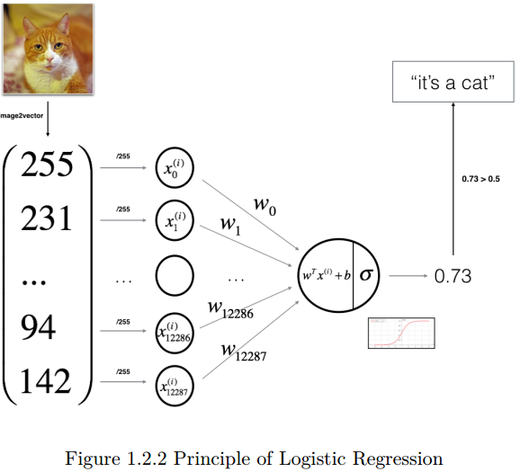
该算法的数学表达:
对于每一个样本x(i):
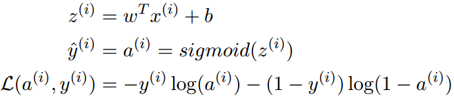
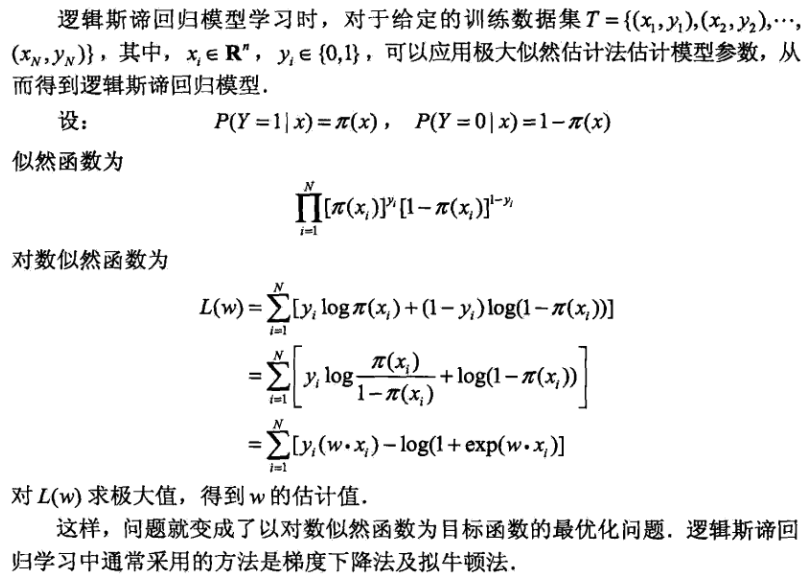
这里的L其实是,每一个样本看做一次伯努利实验,那么分布就是0-1分布,那么对这个0-1分布求极大似然估计就是...贴一波《统计学习方法》的推导:
吴恩达在这里的L函数其实是统计学习方法中的对数似然函数取负的其中一项。
那吴恩达在这里给出的代价函数为:
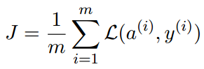
那么可以看到他这个代价函数J其实就是对《统计学习方法》中给出的似然函数取负并归一化了一下(除以m)。
那么接着往下刚。。。
Key steps:
* 初始化模型参数
* 通过最小化代价函数学习模型参数
* 使用学习到的参数来做预测(在测试集上)
* 分析结果并得出结论
1.2.4 Building the parts of our algorithm
构建一个神经网络的主要步骤有:
* 定义模型架构(如输入features的个数)
* 初始化模型参数
* 循环:
- 计算当前的损失(前向传播)
- 计算当前的梯度(反向传播)
- 更新参数(梯度下降)
通常将1-3步分别实现并集成在一个model()函数里。