阅读文档:使用 PyTorch 进行深度学习:60分钟快速入门。
本教程的目标是:
- 总体上理解 PyTorch 的张量库和神经网络
- 训练一个小的神经网络来进行图像分类
PyTorch 是个啥?
这是基于 Python 的科学计算包,其目标是:
- 替换 NumPy,发挥 GPU 的作用
- 一个提供最大灵活性和速度的深度学习研究平台
起步
PyTorch 中的 Tensor 类似于 NumPy 中的 ndarray(这一点类似于 TensorFlow),只不过张量可以充分利用 GPU 来进行加速计算。
1 from __future__ import print_function
2 import torch
构建一个 5*3 的矩阵:
1 x = torch.empty(5, 3)
2 print(x)
tensor([[7.0976e+22, 1.8515e+28, 4.1988e+07],
        [3.0357e+32, 2.7224e+20, 7.7782e+31],
        [4.7429e+30, 1.3818e+31, 1.7225e+22],
        [1.4602e-19, 1.8617e+25, 1.1835e+22],
        [4.3066e+21, 6.3828e+28, 1.4603e-19]])
直接通过数据来构建张量:
1 x = torch.tensor([5.5, 3])
2 print(x)
tensor([5.5000, 3.0000])
还可以根据已有张量来创建张量。这个方法会重用输入张量的属性(例如 dtype)。
1 x = x.new_ones(5, 3, dtype=torch.double)  # new_* methods take in sizes
2 print(x)
3
4 x = torch.randn_like(x, dtype=torch.float)  # override dtype!
5 print(x)                                    # result has the same size
tensor([[1., 1., 1.],
        [1., 1., 1.],
        [1., 1., 1.],
        [1., 1., 1.],
        [1., 1., 1.]], dtype=torch.float64)
tensor([[ 0.4845, -1.2227, -1.2535],
        [ 0.2278,  0.9922,  0.5871],
        [-1.8249,  0.6308,  1.0100],
        [ 0.0126,  0.0591, -0.6153],
        [ 0.1847, -1.8002,  0.7629]])
获取张量的大小:
1 print(x.size())
torch.Size([5, 3])
注意:torch.Size 对象实际上是元组,支持所有元组操作。
运算
PyTorch 支持多种运算语法(类似于 TensorFlow),下面我们看看各种加法的运算。
加法语法 1:
1 y = torch.rand(5, 3)
2 print(x + y)
tensor([[ 1.2256, -0.4395, -0.4990],
        [ 0.4846,  1.7138,  1.0470],
        [-1.3466,  0.7643,  1.0811],
        [ 0.4865,  0.7320, -0.4655],
        [ 0.5111, -1.0667,  1.2088]])
加法语法 2:
1 print(torch.add(x, y))
tensor([[ 1.2256, -0.4395, -0.4990],
        [ 0.4846,  1.7138,  1.0470],
        [-1.3466,  0.7643,  1.0811],
        [ 0.4865,  0.7320, -0.4655],
        [ 0.5111, -1.0667,  1.2088]])
输出张量作为参数的加法:
1 result = torch.empty(5, 3)
2 torch.add(x, y, out=result)
3 print(result)
tensor([[ 1.2256, -0.4395, -0.4990],
        [ 0.4846,  1.7138,  1.0470],
        [-1.3466,  0.7643,  1.0811],
        [ 0.4865,  0.7320, -0.4655],
        [ 0.5111, -1.0667,  1.2088]])
就地(in-place)的加法:
1 y.add_(x)
2 print(y)
tensor([[ 1.2256, -0.4395, -0.4990],
        [ 0.4846,  1.7138,  1.0470],
        [-1.3466,  0.7643,  1.0811],
        [ 0.4865,  0.7320, -0.4655],
        [ 0.5111, -1.0667,  1.2088]])
注意:所有让张量就地发生变化的运算都会在后面加上 _(例如:x.copy_(y)、x.t_())。
随时可以使用类似于 Numpy 的索引操作。
1 print(x[:, 1])
tensor([-1.2227, 0.9922, 0.6308, 0.0591, -1.8002])
如果需要改变张量的形状,使用 torch.view:
1 x = torch.randn(4, 4)
2 y = x.view(16)
3 z = x.view(-1, 8)  # -1 所在的维度通过推断得出
4 print(x.size(), y.size(), z.size())
torch.Size([4, 4]) torch.Size([16]) torch.Size([2, 8])
如果张量只有一个元素,可以通过 .item() 直接获取 Python 数值。
1 x = torch.randn(1)
2 print(x)
3 print(x.item())
tensor([0.2206])
0.22063039243221283
Numpy Bridge
PyTorch 张量和 Numpy 数组之间可以很容易地进行转换。
如果 Tensor 运行在 CPU 上,那么 Tensor 和 NumPy 数组可以共享同一内存。改变内存中的数值会同时影响到 Tensor 和 Numpy 数组。
将 Tensor 转换为 NumPy 数组
1 a = torch.ones(5)
2 print(a)
3 b = a.numpy()
4 print(b)
5 a.add_(1)
6 print(a)
7 print(b)
tensor([1., 1., 1., 1., 1.])
[1. 1. 1. 1. 1.]
tensor([2., 2., 2., 2., 2.])
[2. 2. 2. 2. 2.]
将 NumPy 数组转换为 Tensor
1 import numpy as np
2 a = np.ones(5)
3 b = torch.from_numpy(a)
4 np.add(a, 1, out=a)
5 print(a)
6 print(b)
[2. 2. 2. 2. 2.]
tensor([2., 2., 2., 2., 2.], dtype=torch.float64)
CUDA 张量
使用 .to 方法,张量可以移动到任何设备上(如 CUDA)。
1 # let us run this cell only if CUDA is available
2 # We will use ``torch.device`` objects to move tensors in and out of GPU
3 if torch.cuda.is_available():
4     device = torch.device('cuda')  # 一个 CUDA 设备对象
5     y = torch.ones_like(x, device=device)  # 直接在 GPU 上创建一个张量
6     x = x.to(device)                       # 或者使用 .to('cuda')
7     z = x + y
8     print(z)
9     print(z.to('cpu', torch.double))       # to 也可以同时修改 dtype
tensor([-0.0786], device='cuda:0')
tensor([-0.0786], dtype=torch.float64)
AUTOGRAD:自动求导
在所有 PyTorch 的神经网络中,最核心的就是 autograd 包。我们首先简单了解一下它,其后我们会训练一个自己的神经网络。
autograd 包对于张量的运算提供了自动求导功能。
张量
torch.Tensor 是该包的核心类。如果你设定它的属性 .requires_grad 为 True,那么它会追踪张量的所有运算。结束运算时,调用 .backward() 可以自动计算所有的梯度。该张量的梯度会聚合到 .grad 属性中。
如果需要停止追踪,你需要调用 .detach() 将张量对计算历史解绑,避免后续计算的追踪。
除了上面的方法,你还可以把代码块封装在 with torch.no_grad(): 中。这在评估模型时非常有用,因为模型可能会有 require_grad=True 的参数,但是我们并不需要它们的梯度。
自动求导的实现中,还有一个类非常重要:Function。
Tensor 和 Function 相互关联,构建一张非循环的图,这张图编码了完整的计算历史。每个张量有一个 .grad_fn 属性来引用一个创建该张量的 Function。
如果你需要计算导数,可以调用 Tensor 的 .backward() 方法。
创建一个 requires_grad=True 的张量:
1 x = torch.ones(2, 2, requires_grad=True)
2 print(x)
tensor([[1., 1.],
        [1., 1.]], requires_grad=True)
进行张量运算:
1 y = x + 2
2 print(y)
tensor([[3., 3.],
        [3., 3.]], grad_fn=<AddBackward0>)
y 是运算的结果,因此它有 grad_fn 属性。
1 print(y.grad_fn)
<AddBackward0 object at 0x7f3287a29390>
进行更多运算:
1 z = y * y * 3
2 out = z.mean()
3
4 print(z, out)
tensor([[27., 27.],
        [27., 27.]], grad_fn=<MulBackward0>) tensor(27., grad_fn=<MeanBackward0>)
.requires_grad_(...) 会原地改变当前张量的 requires_grad 标记。
1 a = torch.randn(2, 2)
2 a = ((a * 3) / (a - 1))
3 print(a.requires_grad)
4 a.requires_grad_(True)
5 print(a.requires_grad)
6 b = (a * a).sum()
7 print(b.grad_fn)
False
True
<SumBackward0 object at 0x7f3287a18908>
梯度
让我们进行后馈操作。由于 out 包含一个标量,out.backward() 等价于 out.backward(torch.tensor(1.))。
1 out.backward()
打印梯度 d(out)/dx:
1 print(x)
2 print(out)
3 print(x.grad)
tensor([[1., 1.],
        [1., 1.]], requires_grad=True)
tensor(27., grad_fn=<MeanBackward0>)
tensor([[4.5000, 4.5000],
        [4.5000, 4.5000]])
我们来验证一下这个结果。我们计算的梯度是 $frac{partial out}{partial x_i}$,而
$$out = frac{1}{4}sum z_{i}$$
并且
$$z_i=3 imes y^2=3 imes(x+2)^2$$
因此
$$frac{partial out}{partial x_i}=frac{partial out}{partial z_i}frac{partial z_i}{partial x_i}=frac{1}{4} imes 6(x+2)=frac{3(x+2)}{2}$$
由于 $x_i=1$,代入可以得到
$$frac{partial out}{partial x_i}|_{i=1}=4.5$$
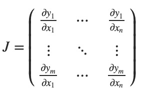
我们在从矩阵的意义上去理解:如果有一个向量函数 $vec{y}=f(vec{x})$,那么 $vec{y}$ 对于 $vec{x}$ 的梯度是一个 Jacobian 矩阵:
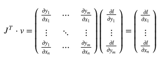
大体上讲,torch.autograd 就是计算向量-Jacobian矩阵的内积的引擎。给定 $v=(v_1, v_2, ..., v_m)^T$,计算内积 $J^Tv$。如果 v 正好是标量函数的梯度 $l=g(vec y)$,即 $v=(frac{partial l}{partial y_1}, ...,frac{partial l}{partial y_m})^T$,那么这个向量-Jacobian矩阵的内积就等于 $l$ 对于 $vec x$ 的导数:
下面看一个向量-Jacobian内积的例子:
1 x = torch.randn(3, requires_grad=True)
2 y = x * 2
3 while y.data.norm() < 1000:
4     y = y * 2
5
6 print(y)
tensor([-886.5914, 41.8782, 1542.3958], grad_fn=<MulBackward0>)
现在由于 y 不是标量,torch.autograd 不能直接计算整个 Jacobian 矩阵。但是如果希望求得向量-Jacobian的内积,可以向 backward 传入一个向量参数。
1 v = torch.tensor([0.1, 1.0, 0.0001], dtype=torch.float)
2 y.backward(v)
3
4 print(x.grad)
tensor([4.0960e+02, 4.0960e+03, 4.0960e-01])
可以用 with torch.no_grad(): 来封装代码块:
1 print(x.requires_grad)
2 print((x ** 2).requires_grad)
3
4 with torch.no_grad():
5     print((x ** 2).requires_grad)
True
True
False
神经网络
我们可以使用 torch.nn 包来构建神经网络。
nn 依赖于 autograd 来定义模型并且对模型求导。nn.Module 包含神经网络层以及一个 forward(input) 方法返回输出。
例如下面分类数字图片的神经网络:
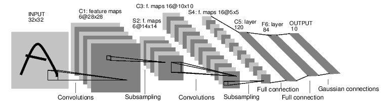
这是一个简单的前馈神经网络。一个神经网络的传统训练方法是:
- 定义含有一些可以学习的参数(或权重)的神经网络。
- 遍历一个输入数据集。
- 将输入向前传入神经网络。
- 计算损失。
- 向后传播梯度到神经网络的参数。
- 更新神经网络的参数,通常使用简单的更新规则: weight = weight - learning_rate * gradient
定义神经网络
 1 import torch
 2 import torch.nn as nn
 3 import torch.nn.functional as F
 4
 5 class Net(nn.Module):
 6
 7     def __init__(self):
 8         super(Net, self).__init__()
 9         # 1 input image channel, 6 output channels, 3x3 square convolution
10         # kernel
11         self.conv1 = nn.Conv2d(1, 6, 3)
12         self.conv2 = nn.Conv2d(6, 16, 3)
13         # an affine operation: y = Wx + b
14         self.fc1 = nn.Linear(16 * 6 * 6, 120)  # 6*6 from image dimension
15         self.fc2 = nn.Linear(120, 84)
16         self.fc3 = nn.Linear(84, 10)
17
18     def forward(self, x):
19         # Max pooling over a (2, 2) window
20         x = F.max_pool2d(F.relu(self.conv1(x)), (2, 2))
21         # If the size is a square you can only specify a single number
22         x = F.max_pool2d(F.relu(self.conv2(x)), 2)
23         x = x.view(-1, self.num_flat_features(x))
24         x = F.relu(self.fc1(x))
25         x = F.relu(self.fc2(x))
26         x = self.fc3(x)
27         return x
28
29     def num_flat_features(self, x):
30         size = x.size()[1:]  # all dimensions except the batch dimension
31         num_features = 1
32         for s in size:
33             num_features *= s
34         return num_features
35
36
37 net = Net()
38 print(net)
Net(
  (conv1): Conv2d(1, 6, kernel_size=(3, 3), stride=(1, 1))
  (conv2): Conv2d(6, 16, kernel_size=(3, 3), stride=(1, 1))
  (fc1): Linear(in_features=576, out_features=120, bias=True)
  (fc2): Linear(in_features=120, out_features=84, bias=True)
  (fc3): Linear(in_features=84, out_features=10, bias=True)
)
这里我们定义了 forward 函数,而 backward 函数(计算梯度)可以使用 autograd 自动定义。
学习好的模型参数可以通过 net.parameters() 返回。
1 params = list(net.parameters())
2 print(len(params))
3 print(params[0].size())  # conv1's .weight
10
torch.Size([6, 1, 3, 3])
接下来我们尝试随机的 32*32 输入(LeNet 所设置的输入大小是 32*32)。
1 input = torch.randn(1, 1, 32, 32)
2 out = net(input)
3 print(out)
tensor([[-0.0236, -0.0104,  0.0173, -0.1874, -0.0613, -0.0162, -0.1466,  0.1535,
          0.0596, -0.0320]], grad_fn=<AddmmBackward>)
在进一步学习之前,这里再回顾一下你看过的类。
- torch.Tensor:支持自动求导运算(backward())的多维数组。同时它也保存着梯度信息。
- nn.Module:神经网络模块。可以很容易地封装参数、放到 GPU 进行运算、导出和加载等。
- nn.Parameter:某种张量,当赋值为 Module 的属性时,可以自动注册为参数。
- autograd.Function:实现自动求导运算的前馈和后馈的定义。每个 Tensor 运算会创建至少一个 Function 节点(创建该 Tensor 的函数)。
到目前为止,我们讲解了:
- 定义一个神经网络
- 处理输入并且调用后馈运算
我们还需要:
- 计算损失(loss)
- 更新神经网络的权重
损失函数
损失函数接收输入的 (output, target) 对,计算出 output 与 target 之间的差值。
在 nn 包中有很多不同的损失函数。 最简单的是 nn.MSELoss,计算出两者的均方误差。
1 output = net(input)
2 target = torch.randn(10)  # a dummy target, for example
3 target = target.view(1, -1)  # make it the same shape as output
4 criterion = nn.MSELoss()
5
6 loss = criterion(output, target)
7 print(loss)
tensor(0.6006, grad_fn=<MseLossBackward>)
我们可以查看反向传播的各层的运算:
1 print(loss.grad_fn)  # MSELoss
2 print(loss.grad_fn.next_functions[0][0])  # Linear
3 print(loss.grad_fn.next_functions[0][0].next_functions[0][0])  # ReLU
<MseLossBackward object at 0x7f3280404588>
<AddmmBackward object at 0x7f32804047f0>
<AccumulateGrad object at 0x7f3280404588>
反向传播
我们使用 loss.backward() 进行误差的反向传播。但是你需要清除现有的梯度,否则梯度会已存在的梯度上累积。
我们调用 loss.backward(),并且观察 conv1 的偏差的梯度的变化。
1 net.zero_grad()  # zeroes the gradient buffers of all parameters
2
3 print('conv1.bias.grad before backward')
4 print(net.conv1.bias.grad)
5
6 loss.backward()
7
8 print('conv1.bias.grad after backward')
9 print(net.conv1.bias.grad)
conv1.bias.grad before backward
None
conv1.bias.grad after backward
tensor([ 3.5922e-03,  7.0686e-03,  3.9444e-03,  1.1225e-02, -5.1291e-03,
        -6.0605e-05])
权重的更新
实践中最简单的更新方法是随机梯度下降(Stochastic Gradient Descent, SGD):
weight = weight - learning_rate * gradient
我们可以用简单的 Python 代码来实现:
1 learning_rate = 0.01
2 for f in net.parameters():
3     f.data.sub_(f.grad.data * learning_rate)
然而,使用神经网络的时候,你可能会使用不同的更新方法(SGD、Nesterov-SGD、Adam、RMSProp 等)。为了满足这方面的需求,PyTorch 构建了一个包:torch.optim 实现了所有这些方法。
 1 import torch.optim as optim
 2
 3 # create your optimizer
 4 optimizer = optim.SGD(net.parameters(), lr=0.01)
 5
 6 # in your training loop:
 7 optimizer.zero_grad()  # zero the gradient buffers
 8 output = net(input)
 9 loss = criterion(output, target)
10 loss.backward()
11 optimizer.step()  # Does the update
训练一个分类器
前面我们已经可以定义神经网络、计算损失并且更新神经网络的权重了。
那么什么是数据?
通常,当处理图像、文本、音频或者视频数据时,你可以使用标准 Python 包来将数据加载为 Numpy 数组。接着你可以把 NumPy 数组转换为 torch.*Tensor。
- 对于图片,可能使用 Pillow/OpenCV 这些包
- 对于音频,可能使用 scipy/librosa 这些包
- 对于文本,可以使用 Python/Cython/NLTK/SpaCy 进行处理
对于计算机视觉,PyTorch 提供了一个叫 torchvision 的包,可以加载常见的数据集(imagenet/CIFAR10/MNIST 等),对图片进行数据转换。
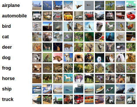
在这里,我们会使用 CIFAR10 数据集。它有这几个种类:airplane, automobile, bird, cat, deer, dog, frog, horse, ship, truck。CIFAR-10 的图片大小都是 3*32*32。
训练图片分类器
我们的步骤是这样的:
- 使用 torchvision 加载并且标准化 CIFAR10 的训练接和数据集。
- 定义一个卷积神经网络。
- 定义损失函数。
- 在训练集上训练神经网络。
- 在测试集上训练神经网络。
1. 加载并标准化 CIFAR10
使用 torchvision,要加载 CIFAR10 很容易。
1 import torch
2 import torchvision
3 import torchvision.transforms as transforms
torchvision 数据集的输出是范围 0~1 的 PIL 图片。我们将它标准化,范围 -1~1。
 1 transform = transforms.Compose([
 2     transforms.ToTensor(),
 3     transforms.Normalize((0.5, 0.5, 0.5), (0.5, 0.5, 0.5))
 4 ])
 5
 6 trainset = torchvision.datasets.CIFAR10(root='./data', train=True, download=True, transform=transform)
 7 trainloader = torch.utils.data.DataLoader(trainset, batch_size=4, shuffle=True, num_workers=2)
 8 testset = torchvision.datasets.CIFAR10(root='./data', train=False, download=True, transform=transform)
 9 testloader = torch.utils.data.DataLoader(testset, batch_size=4, shuffle=False, num_workers=2)
10 classes = ('plane', 'car', 'bird', 'cat', 'deer', 'dog', 'frog', 'horse', 'ship', 'truck')
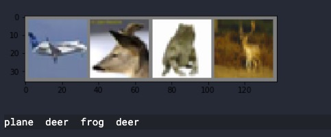
下面显示部分训练图片:
 1 import matplotlib.pyplot as plt
 2 import numpy as np
 3
 4 # functions to show an image
 5
 6
 7 def imshow(img):
 8     img = img / 2 + 0.5     # unnormalize
 9     npimg = img.numpy()
10     plt.imshow(np.transpose(npimg, (1, 2, 0)))
11     plt.show()
12
13
14 # get some random training images
15 dataiter = iter(trainloader)
16 images, labels = dataiter.next()
17
18 # show images
19 imshow(torchvision.utils.make_grid(images))
20 # print labels
21 print(' '.join('%5s' % classes[labels[j]] for j in range(4)))
2. 定义卷积神经网络
 1 import torch.nn as nn
 2 import torch.nn.functional as F
 3
 4 class Net(nn.Module):
 5     def __init__(self):
 6         super(Net, self).__init__()
 7         self.conv1 = nn.Conv2d(3, 6, 5)
 8         self.pool = nn.MaxPool2d(2, 2)
 9         self.conv2 = nn.Conv2d(6, 16, 5)
10         self.fc1 = nn.Linear(16 * 5 * 5, 120)
11         self.fc2 = nn.Linear(120, 84)
12         self.fc3 = nn.Linear(84, 10)
13
14     def forward(self, x):
15         x = self.pool(F.relu(self.conv1(x)))
16         x = self.pool(F.relu(self.conv2(x)))
17         x = x.view(-1, 16 * 5 * 5)
18         x = F.relu(self.fc1(x))
19         x = F.relu(self.fc2(x))
20         x = self.fc3(x)
21         return x
22
23 net = Net()
24 print(net)
Net(
  (conv1): Conv2d(3, 6, kernel_size=(5, 5), stride=(1, 1))
  (pool): MaxPool2d(kernel_size=2, stride=2, padding=0, dilation=1, ceil_mode=False)
  (conv2): Conv2d(6, 16, kernel_size=(5, 5), stride=(1, 1))
  (fc1): Linear(in_features=400, out_features=120, bias=True)
  (fc2): Linear(in_features=120, out_features=84, bias=True)
  (fc3): Linear(in_features=84, out_features=10, bias=True)
)
3. 定义损失函数和优化器
我们使用分类交叉熵和动量 SGD。
1 import torch.optim as optim
2
3 criterion = nn.CrossEntropyLoss()
4 optimizer = optim.SGD(net.parameters(), lr=0.001, momentum=0.9)
4. 训练网络
 1 %%time
 2 for epoch in range(4):  # loop over the dataset multiple times
 3
 4     running_loss = 0.0
 5     for i, data in enumerate(trainloader, 0):
 6         # get the inputs; data is a list of [inputs, labels]
 7         inputs, labels = data
 8
 9         # zero the parameter gradients
10         optimizer.zero_grad()
11
12         # forward + backward + optimize
13         outputs = net(inputs)
14         loss = criterion(outputs, labels)
15         loss.backward()
16         optimizer.step()
17
18         # print statistics
19         running_loss += loss.item()
20         if i % 2000 == 1999:    # print every 2000 mini-batches
21             print('[%d, %5d] loss: %.3f' %
22                   (epoch + 1, i + 1, running_loss / 2000))
23             running_loss = 0.0
24
25 print('Finished Training')
[1,  2000] loss: 2.223
[1,  4000] loss: 1.949
[1,  6000] loss: 1.754
[1,  8000] loss: 1.622
[1, 10000] loss: 1.544
[1, 12000] loss: 1.496
[2,  2000] loss: 1.412
[2,  4000] loss: 1.386
[2,  6000] loss: 1.373
[2,  8000] loss: 1.335
[2, 10000] loss: 1.327
[2, 12000] loss: 1.295
[3,  2000] loss: 1.221
[3,  4000] loss: 1.239
[3,  6000] loss: 1.255
[3,  8000] loss: 1.193
[3, 10000] loss: 1.186
[3, 12000] loss: 1.203
[4,  2000] loss: 1.126
[4,  4000] loss: 1.140
[4,  6000] loss: 1.120
[4,  8000] loss: 1.122
[4, 10000] loss: 1.112
[4, 12000] loss: 1.114
Finished Training
CPU times: user 3min 34s, sys: 45.6 s, total: 4min 20s
Wall time: 4min 49s
5. 在测试集上测试网络
我们对神经网络训练了 2 次,接下来要看一下该网络是否学习到了东西。
首先展示测试集的几张图片。
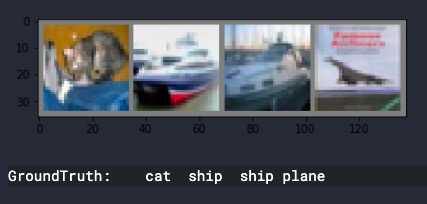
接下来让我们看一下神经网络认为这几张图片是啥。
1 _, predicted = torch.max(outputs, 1)
2
3 print('Predicted: ', ' '.join('%5s' % classes[predicted[j]] for j in range(4)))
Predicted: cat ship plane car
结果看起来还凑合。
接下来我们看一下在整个测试集上神经网络表现得如何。
 1 correct = 0
 2 total = 0
 3 with torch.no_grad():
 4     for data in testloader:
 5         images, labels = data
 6         outputs = net(images)
 7         _, predicted = torch.max(outputs.data, 1)
 8         total += labels.size(0)
 9         correct += (predicted == labels).sum().item()
10
11 print('Accuracy of the network on the 10000 test images: %d %%' % (100 * correct / total))
Accuracy of the network on the 10000 test images: 58 %
再看看每个分类下的表现:
 1 class_correct = list(0. for i in range(10))
 2 class_total = list(0. for i in range(10))
 3 with torch.no_grad():
 4     for data in testloader:
 5         images, labels = data
 6         outputs = net(images)
 7         _, predicted = torch.max(outputs, 1)
 8         c = (predicted == labels).squeeze()
 9         for i in range(4):
10             label = labels[i]
11             class_correct[label] += c[i].item()
12             class_total[label] += 1
13
14
15 for i in range(10):
16     print('Accuracy of %5s : %2d %%' % (
17         classes[i], 100 * class_correct[i] / class_total[i]))
Accuracy of plane : 63 %
Accuracy of   car : 73 %
Accuracy of  bird : 50 %
Accuracy of   cat : 41 %
Accuracy of  deer : 31 %
Accuracy of   dog : 47 %
Accuracy of  frog : 79 %
Accuracy of horse : 60 %
Accuracy of  ship : 77 %
Accuracy of truck : 64 %
在 GPU 上进行训练
就像之前我们把张量放到 GPU 上一样,我们需要把神经网络也放在 GPU。
如果我们有 CUDA,先定义设备:
1 device = torch.device('cuda:0' if torch.cuda.is_available() else 'cpu')
2
3 # Assuming that we are on a CUDA machine, this should print a CUDA device:
4 print(device)
cuda:0
查看可以使用的 GPU 数量:
1 print(torch.cuda.device_count())
1
然后注意把模型和输入数据放入 GPU 进行训练:
 1 %%time
 2 net.to(device)
 3 for epoch in range(4):  # loop over the dataset multiple times
 4
 5     running_loss = 0.0
 6     for i, data in enumerate(trainloader, 0):
 7         # get the inputs; data is a list of [inputs, labels]
 8         inputs, labels = data
 9         inputs, labels = inputs.to(device), labels.to(device)
10
11         # zero the parameter gradients
12         optimizer.zero_grad()
13
14         # forward + backward + optimize
15         outputs = net(inputs)
16         loss = criterion(outputs, labels)
17         loss.backward()
18         optimizer.step()
19
20         # print statistics
21         running_loss += loss.item()
22         if i % 2000 == 1999:    # print every 2000 mini-batches
23             print('[%d, %5d] loss: %.3f' %
24                   (epoch + 1, i + 1, running_loss / 2000))
25             running_loss = 0.0
26
27 print('Finished Training')
[1,  2000] loss: 2.225
[1,  4000] loss: 1.895
[1,  6000] loss: 1.678
[1,  8000] loss: 1.565
[1, 10000] loss: 1.508
[1, 12000] loss: 1.467
[2,  2000] loss: 1.393
[2,  4000] loss: 1.349
[2,  6000] loss: 1.319
[2,  8000] loss: 1.317
[2, 10000] loss: 1.322
[2, 12000] loss: 1.255
[3,  2000] loss: 1.191
[3,  4000] loss: 1.200
[3,  6000] loss: 1.230
[3,  8000] loss: 1.190
[3, 10000] loss: 1.162
[3, 12000] loss: 1.167
[4,  2000] loss: 1.096
[4,  4000] loss: 1.102
[4,  6000] loss: 1.089
[4,  8000] loss: 1.099
[4, 10000] loss: 1.092
[4, 12000] loss: 1.066
Finished Training
CPU times: user 2min 27s, sys: 20.2 s, total: 2min 47s
Wall time: 3min 33s
加速效果跟神经网络的大小有关系,不适用 GPU 需要 4 分 49 秒,我们的 GPU 版本消耗时间 3 分 33 秒。我们目前的神经网络还比较小,因此加速效果并不是非常大。