ABSTRACT
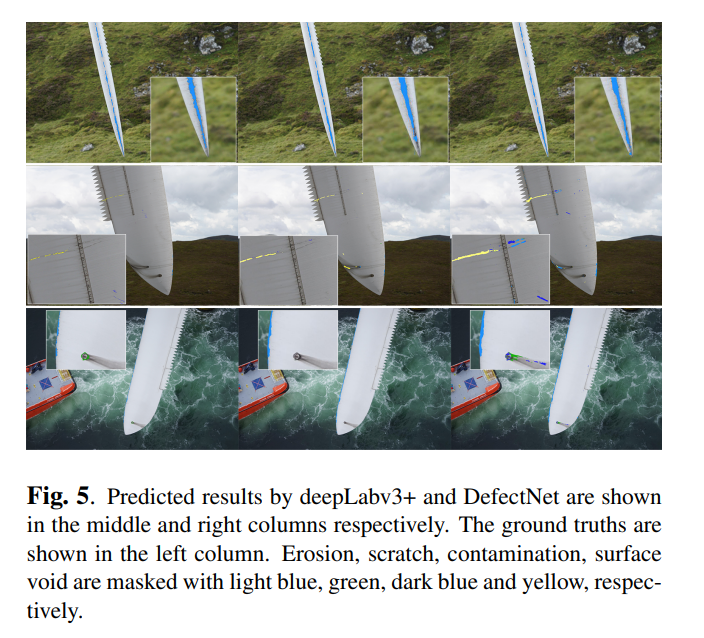
As a data-driven method, the performance of deep convolutional neural networks (CNN) relies heavily on training data. The prediction results of traditional networks give a bias toward larger classes, which tend to be the background in the semantic segmentation task. This becomes a major problem for fault detection, where the targets appear very small on the images and vary in both types and sizes. In this paper we propose a new network architecture, DefectNet, that offers multiclass (including but not limited to) defect detection on highlyimbalanced datasets. DefectNet consists of two parallel paths, which are a fully convolutional network and a dilated convolutional network to detect large and small objects respectively. We propose a hybrid loss maximising the usefulness of a dice loss and a cross entropy loss, and we also employ the leaky rectified linear unit (ReLU) to deal with rare occurrence of some targets in training batches. The prediction results show that our DefectNet outperforms state-of-the-art networks for detecting multi-class defects with the average accuracy improvement of approximately 10% on a wind turbine.
摘要
一个样本驱使的方法,深度卷积神经网络的效果嫉妒依赖训练数据,传统网络的预测结果对于较大的类别具有偏置,在语义分割中的任务倾向于背景。对于故障检测这将变成一个主要的问题,在图像中的目标是非常小而且有不同的类型和尺寸。在这篇文章中我们采用了一个新的网络结构,缺陷网络,在极度不平衡的数据集上,它提供了多类别(包括但不限制的)缺陷检测。缺陷网络包含两个平行路径,一个是全卷积网络和一个空洞卷积网络分别去发现大和小目标。我们采用了一个混合损失最大化利用距离损失和交叉熵损失,同样我们也使用漏整流线型单元(LReLU)去解决在训练批次中少量出现的目标。这个预测结果显示我们的DefectNet表现出最好的网络,对于检测多类型的缺陷平均结果提升了10%在风车涡轮上。
INTRODUCTION
Numerous approaches have been proposed to create balanced distributions of data using data manipulation [2]. These include downsampling majority classes, oversampling minority classes, or both. However, for semantic segmentation, augmenting the number of samples in the smaller classes always includes more of the surrounding areas, resulting in more samples of the larger class too – augmenting the small classes always add more background samples. Hence we employ the other techniques that deal with the imbalanced training data issue by modifying the network architecture and the validation loss.
介绍
很多方法被提出使用数据操作来生成平衡的数据分布,这就包括主要类别的降采样,过采样小数类,或者两者都用。然而,对于语义分割,在小类别增加样本的数量包含更多的周边区域,导致了大样本的数量也更多。增加小样本的类别总是会添加更多的背景样本。因此我们采用其他的方法通过修饰网络结构和校准损失来解决不平衡训练数据的问题。
For convolutional neural networks (CNNs), classical techniques balance classes using weights computed by analysing dataset statistics. A dice coefficient-based loss has been employed by Milletari et al. [3], giving better segmentation results than re-weighted soft-max with loss. Later, the generalised dice loss was proposed for multiple classes by Sudre et al. [4]. Although the dice loss has become popular for medical imaging tasks, the cross entropy loss has been reported to have better performance in some applications [5]. Recently he ideas of combined loss have been introduced [6, 7]. However none of these approaches have been tested in a challenging scenario, such as defect detection, where each training batch does not contain all class samples.
对于卷积神经网络,典型技术是使用统计分析数据计算得到的权重来平衡类别。一个基于距离系数的损失已经被应用在Milletari et al. 给了更好的分割结果超过重新加权softmax损失。最后,Sudre提出了多类别的全面距离损失。尽管距离损失在医疗图片上变得流行,交叉熵已经被证实在一些应用上表现的更好。最近,融合两种损失函数的想法已经被提出。然而没有任何方法已经在一个有挑战的场景下被测试,比如缺陷检测,这里的一个训练batch不能包含所有类别样本。
Another problem when detecting small objects using CNNs is the decrease of receptive field size as the network depth increases. CNNs used for classification employ a pooling layer after the convolutional layer to combine the outputs of neuron clusters from one layer into a single neuron in the next layer. This results in feature maps with reduced spatial resolution with the outcome that very small areas could be represented by only one pixel. Dilated convolutional layers have therefore been introduced to enlarge the field of view of the filters [8]. Generally the dilation rate of the filter size (inserting more zeros) increases with larger depth. However this can cause false positives for small classes [9]. We therefore diminish this problem here by combining feature maps from traditional convolutional layers with dilated convolutional layers.
另外一个问题,当使用CNN去发现小目标物体时,是接受域的尺寸随着网络深度的加深不断减少。CNNs被用来分类在一个卷积层之后使用池化层,将输出的神经元集群合并到下一层的一个简单神经元。在特征图上的结果通过减少空间分辨率导致非常小的面积可能会被表达成只有单个像素。空洞卷积层因此被用来扩大过滤器的感受野。通常降低过滤器的尺寸增加更大的深度。然后对于小类别的物体,这将会引入更多的假阳性。因此我们将传统的卷积层融合空洞卷积层来降低这个问题。
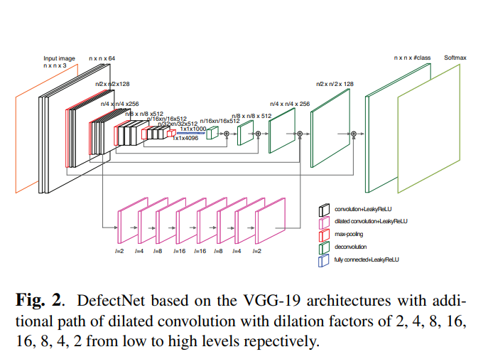
In this paper, we propose a new network, DefectNet, for detecting various defect size on a highly imbalanced dataset. The proposed DefectNet, shown in Fig. 2, has two parallel paths, where one of them makes use of skip layers [1] to detect medium to large objects. The additional path employs the dilated convolutional layers to increase receptive field size for small object defect detection. The two paths are combined with sum fusion at the construction end. We also propose a hybrid loss function that combines the advantages of the cross entropy and dice losses. The cross entropy loss compensates for some absent classes in the training batches, whilst the dice loss improves the balance between the precision and recall. We employ LeakyReLU (Leaky rectified linear unit) to prevent zero gradients when some small classes are not included in several training batches consecutively.
在这篇文章中,我们提出了一个新的网络,缺陷网络,在一个极高不平衡的数据中检测不同缺陷尺寸。这个提出的缺陷网络,在Fig.2中被显示,有两个并行路径,其中一个使用跳层结构去发现中型或者大型物体。这个额外的路径采用了一个空洞卷积层去增加小物体缺陷检测接受域的尺寸。这两个路径在架构的结尾进行融合。我们也采用一个混合损失函数融合交叉熵损失和距离损失的优势。交叉熵损失在训练batch中补偿很多缺失的类别,然而距离损失改善准确率和召回率的平衡。当一些小的类别在几个连续训练batches中没有被包含时, 我们采用LeakyRelu(漏型流线型单元)去预防零梯度。
这片文章主要的优化点:
1. Dilated convolution(空洞卷积)
2. Hybrid loss(混合损失)
3. Leaky rectified linear unit(LRelu)
DEFECTNET
The architecture of DefectNet is illustrated in Fig. 2. It combines two paths able to detect different target sizes. The first path makes use of the VGG-19 architecture and skip layer fusion creating fully convolutional network. It is an enhanced version of the architecture of the FCN-8 network [1], introducing additional skip layers in pool1 and pool2 in order to include the low-level features for finer prediction. The second path employs the dilated convolution (further described in Section 2.1) to detect the small objects. All filters of the convolutional layers have a kernel size of 3×3, but those of the second path have zero-inserts to create dilated convolution. All convolution processes operate with the stride of 1. The following subsections highlight the differences of the proposed deep learning network to the traditional ones.
缺陷网络的架构在Fig2做展示,它融合了两条路径去发现不同的目标尺寸。第一条路径使用VGG-19结构和跳过层融合生成一个全卷积网络。是FCN-8网络结构的升级版,介绍了第一个池化和第二个池化额外的跳过层, 为了提取在更精细的预测中低语义特征。第二条线采用空洞卷积(在2.1节有更多的说明)去发现更小的物体。所有卷积层的过滤器采用3x3的核尺寸,但是第二条路插入0去生成空洞卷积。所有卷积过程都是用stride等于1进行处理。下面章节着重展示了提出的深度学习网络与传统网络的不同之处。
Dilated convolution
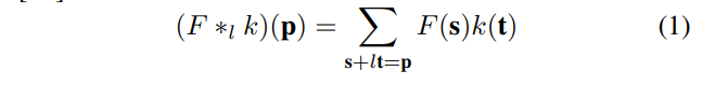
Dilated convolution, also referred to as atrous convolution, enlarges the field of view of the filters to incorporate larger context by expanding the receptive field without loss of resolution. The dilated convolutions are defined in Eq.1 [14], where F is a feature map, k is a filter, l is a convolution operator with a dilation factor l, meaning (l−1) zeros are inserted. We construct eight dilated convolution layers (coloured pink in Fig. 2) after the second group of convolutional layers of the other FCN path. The dilation factor l is defined in Fig. 2. This structure is similar to the basic context network architecture proposed in [14], but we add more dilated convolution layers with decreasing l. This improves local low-level features, where spatial relationships amongst adjacent pixels may be ignored due to sparsity of the dilated filters when increasing l [15].
膨胀卷积
膨胀卷积也被称为空洞卷积,放大滤镜的视场来容纳更大的场景,通过扩大感受野而不损失分辨率。这个膨胀卷积在Eq1里面被定义,这里的F是一个特征图,K是一个过滤器,I是一个带有膨胀因子的卷积核。意味着0被插入。在另外一条FCN路径下的第二组卷积层,我们构造了8个膨胀卷积层。卷积因子l在Fig 2中定义。这个结构与14中提出的基础语义网络结构相似,但是我们加入了更多的膨胀卷积和减少l,这改善了局部的低语义特征,由于膨胀卷积的稀疏性,当增加l参数时,相邻像素的空间联系可能会被忽视。
Hybrid loss
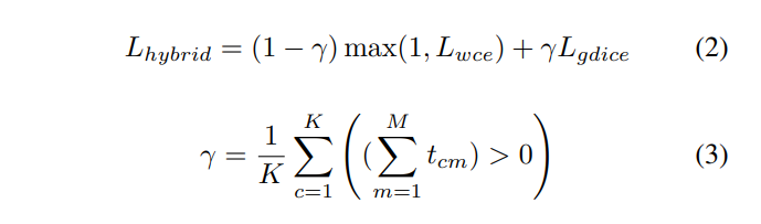
The most commonly used loss function for the task of image segmentation is a pixel-wise cross entropy loss. The class weighting technique is employed to balance the classes to improve training. Another popular loss is the dice loss. The dice coefficient performs better on class imbalanced problems because it maximises a metric that directly measures the region intersection over union. The gradients of the dice coefficients are however not as smooth as those of cross entropy, particularly when both predictions and labels are close to zero. For our dataset, the data in each batch do not contain all classes, leading to very noisy training error. The cross entropy loss, on the other hand, allows the absent classes to affect the backpropagation less than the dice loss. Therefore we propose the hybrid loss defined in Eq. 2, where the weighted cross entropy loss Lwce and generalised dice loss Lgdice are merged in the proportion of the number of class samples present in the training batch (Eq. 3).
混合损失
对于图像分割任务,很多普遍使用的损失时像素级别的交叉熵损失。采用类别加权技术平衡类别,以此改善训练。另外一个流行的损失是距离loss,这个距离系数在类别失衡问题上表现的更好,因为它最大化了直接测量区域交集而非并集的因子。然而dice因素的梯度没有像cross entropy一样平滑,尤其当预测和label趋向于0时。对于我们的数据集,这个数据在每一个batch不能包含所有的类别,引入了非常噪声的训练错误。在另一方面,交叉损失函数允许缺失类别对反向梯度的影响小于dice loss。因此我们采用混合损失,加权交叉熵损失(Lwce)和广义骰子损失被合并到训练批次内。
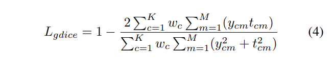
The loss Lwce is definded as Lwce = − PK c=1 wctclog(yc), where K is the number of classes and yc and tc represent the prediction and target, respectively. Generally the weights are computed from pixel counts, i.e. a weight of class c is wc = 1/fc, where fc is pixel counts of class c [16]. However applications such as defect detection have highly-imbalanced classes. Their scores could approach zero and cause poor performance because significantly higher weight values are given to the smaller classes. We hence propose to use wc = 1/ √ fc. Equation 4 shows the generalized dice loss proposed in [4], where ycm and tcm represent the prediction and groundtruth of the pixel m from the total M pixels. The weight in the generalized dice loss is generally calculated as the inverse of the squared sum of all pixels of class c, but this will give priority to the small and absent classes. Therefore in DefectNet, we adapt the dice loss with the same wc used in Lwce.
代码如下:上面的作者并没有放出y的代码
class_weight = tf.constant([0.0013,    0.0012,    0.0305,    0.0705,    0.8689,    0.2045,    0.0937,    0.8034,    0.0046,    0.1884,    0.1517,    0.5828,    0.0695, 0.0019]) #1/freq^(1/3) 类别加权
weights = tf.gather(class_weight, labels)
loss1 = tf.reduce_mean((tf.losses.sparse_softmax_cross_entropy(logits=logits, labels=labels, weights=weights)))
loss2 = generalised_dice_loss(prediction=logits,ground_truth=labels)
loss = tf.minimum(loss1,loss2)
这个Lwce被定义为c=1的wctclog损失,这里K是类别的数量以及yc和tc分别代表了预测值和目标。通常这个损失通过像素进行计算,权重的类别wc = 1/fc,这里的fc是类别的c的像素计算。然而像缺陷检测的应用有高度不平衡的类别。这个分数可能接近0并且造成差的表现因为较小的类别得到了更多的权重值。因此我们提出使用wc = 1/ √ fc. Equation 4显示了在[4]中被提出的广义的dice loss,这里ycm和tcm代表了从M总数中获得的预测值和真实值的像素m。在广义dice损失的权重一般计算为c类所有像素平方和的倒数,但是这对于小样本和缺失样本是有优势的。因此在DefectNet,我们采用与Lwce相同的wc来调整dice损失。
代码如下:
def generalised_dice_loss(prediction,
                          ground_truth,
                          weight_map=None,
                          type_weight='Square'):
    """
    Function to calculate the Generalised Dice Loss defined in
        Sudre, C. et. al. (2017) Generalised Dice overlap as a deep learning
        loss function for highly unbalanced segmentations. DLMIA 2017
    :param prediction: the logits
    :param ground_truth: the segmentation ground truth
    :param weight_map:
    :param type_weight: type of weighting allowed between labels (choice
        between Square (square of inverse of volume),
        Simple (inverse of volume) and Uniform (no weighting))
    :return: the loss
    """
    prediction = tf.cast(prediction, tf.float32)
    if len(ground_truth.shape) == len(prediction.shape):
        ground_truth = ground_truth[..., -1]
    one_hot = labels_to_one_hot(ground_truth, tf.shape(prediction)[-1])
    if weight_map is not None:
          n_classes = prediction.shape[1].value
        weight_map_nclasses = tf.reshape(
            tf.tile(weight_map, [n_classes]), prediction.get_shape())
        ref_vol = tf.sparse_reduce_sum(
            weight_map_nclasses * one_hot, reduction_axes=[0])
        intersect = tf.sparse_reduce_sum(
            weight_map_nclasses * one_hot * prediction, reduction_axes=[0])
        seg_vol = tf.reduce_sum(
            tf.multiply(weight_map_nclasses, prediction), 0)
    else:
        ref_vol = tf.sparse_reduce_sum(one_hot, [0,1,2])
        intersect = tf.sparse_reduce_sum(one_hot * prediction, [0,1,2])
        seg_vol = tf.reduce_sum(prediction, [0,1,2])
    if type_weight == 'Square':
        weights = tf.reciprocal(tf.square(ref_vol))
    elif type_weight == 'Simple':
        weights = tf.reciprocal(ref_vol)
    elif type_weight == 'Uniform':
        weights = tf.ones_like(ref_vol)
    elif type_weight =='Fixed':
        weights = tf.constant([0.0006, 0.0006, 0.1656, 0.1058, 0.0532, 0.0709, 0.1131, 0.3155, 0.1748])  #W3 = 1/sqrt(freq)
    else:
        raise ValueError("The variable type_weight "{}""
                         "is not defined.".format(type_weight))
    new_weights = tf.where(tf.is_inf(weights), tf.zeros_like(weights), weights)
    weights = tf.where(tf.is_inf(weights), tf.ones_like(weights) * tf.reduce_max(new_weights), weights)

    generalised_dice_numerator = 2 * tf.reduce_sum(tf.multiply(weights, intersect))
    generalised_dice_denominator = tf.reduce_sum(tf.multiply(weights, tf.maximum(seg_vol + ref_vol, 1)))
    # generalised_dice_denominator = tf.reduce_sum(tf.multiply(weights, seg_vol + ref_vol)) + 1e-6
    generalised_dice_score = generalised_dice_numerator / generalised_dice_denominator
    generalised_dice_score = tf.where(tf.is_nan(generalised_dice_score), 1.0, generalised_dice_score)

    return 1 - generalised_dice_score
Leaky rectified linear unit
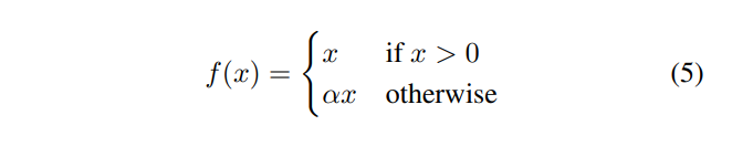
because an entire dataset cannot be fed into the neural network at once, it is divided into multiple batches with random data selection. This means some classes may not present in particular batches, causing some nodes within the layers to have an activation of zero. The backpropogation process does not update the weights for these nodes because their gradient is also zero. This is called the ‘dying ReLU’ problem. To prevent this, we employ the leaky ReLU activation function. It allows a small gradient when the unit is not active (negative inputs) so that the backpropogation will always update the weights. The leaky ReLU is defined as shown in Eq. 5 [17] and α is set to 0.1 during training.
漏整流线型单元
因为整个数据被一次性喂到神经网络中,使用随机数据选择被切分成多个批次。这就意味着某些类不会出现在特定的批处理中,使得层中的一些节点激活值为0。对于这些节点梯度回传不能更新权重,因为这个梯度也是0。这被称为激活层死亡问题。为了防止这个情况,我们采用漏整形激活功能。它允许当这个单元没有被激活的时候是一个很小的梯度。因此回传时总是会更新梯度。这个Leaky Relu被展示在Eq.5并且a被设置为0.1在训练的时候。
上述的代码来自于GitHub - pui-nantheera/DefectNet