POMDP

本文转自：http://www.pomdp.org/

一、Background on POMDPs

　　We assume that the reader is familiar with the value iteration algorithm for regular discrete Markov decision processes (MDPs). However, we will need to differentiate these from POMDPs which we could also call a discrete Markov decision process. Therefore, we will refer to the more familiar MDPs as CO-MDPs, emphasizing that they are completely observable.

　　Adding partial observability to an MDP is not a trivial addition. Solution procedures for CO-MDPs give values or policies for each state. Use of these solutions requires the state to be completely known at all times and with complete observability this presents no problem. Partial observability clouds the idea of the current state. No longer is there certainty about the current state which makes selecting actions based on the current state (as in a CO-MDP) no longer valid.

　　A POMDP is really just an MDP; we have a set of states, a set of actions, transitions and immediate rewards. The actions' effects on the state in a POMDP is exactly the same as in an MDP. The only difference is in whether or not we can observe the current state of the process. In a POMDP we add a set of observations to the model. So instead of directly observing the current state, the state gives us an observation which provides a hint about what state it is in. The observations can be probabilistic; so we need to also specify an observation function. This observation function simply tells us the probability of each observation for each state in the model. We can also have the observation likelihood depend on the action if we like.

　　Although the underlying dynamics of the POMDP are still Markovian, since we have no direct access to the current state, our decisions require keeping track of (possibly) the entire history of the process, making this a non-Markovian process. The history at a given point in time is comprised of our knowledge about our starting situation, all actions performed and all observations seen.

　　Fortunately, it turns out that simply maintaining a probability distribution over all of the states provides us with the same information as if we maintained the complete history. In a CO-MDP we track our current state and update it after each action. Here this is trivial, because it is completely observable. In a POMDP we have to maintain this probability distribution over states. When we perform and action and make an observation, we have to update the distribution. Updating the distribution is very easy and just involves using the transition and observation probabilities. You'll have to take our word for this, since we are prohibited from showing you the formula.

二、Basics of Solving POMDPs

 

　　In this section we finally start to get to the heart of the matter. We will start to introduce the graphical representation we use and then explain how we can use the value iteration algorithm to solve a POMDP problem. Once this is established, we can delve into the particular algorithms that have been used to solve POMDPs.

　　In CO-MDPs our problem is to find a mapping from states to actions; in POMDPs our problem is to find a mapping from probability distributions (over states) to actions. We will refer to a probability distribution over states as a belief state and the entire probability space (the set of all possible probability distributions) as the belief space.（在CO-MDP中，我们寻求的是从状态到动作的一个映射（即策略），在POMDP中我们寻求的是从belief state（指的是对所有状态的概率分布）到动作的一个映射（策略））

　　The figure below introduces how we will represent the belief space. To keep things as simple as possible, we will use a two state POMDP as our running example. For a two state POMDP we can represent the belief state with a single number. Since a belief state is a probability distribution, the sum of all probabilities must sum to 1. With a two state POMDP, if we are given the probability for being in one of the states as being 'p', then we know that the probability of being in the other state must be '1-p'. Therefore the entire space of belief states can be represented as a line segment. The figure below shows this, though we have made the line segment have a significant width.（这里是一个POMDP的简单例子，这个POMDP 只有两个状态，这里是状态分布符合二项分布）

1D belief space for a 2 state POMDP

The thickness of this line will serve only to help clarify later explanations; the belief space is a single line segment. The belief space is labeled with a 0 on the left and a 1 on the right. This is the probability we are in state s1. To the far left(最左端) is the belief state where there is no chance that we are in state s1, which means that we are certain (probability = 1) that we are in state s2. The far right is when we are certain we are in state s1 with no chance of being in state s2. Note that although all of our examples use a two state problem, all of the insights directly apply for higher dimensional spaces; lines in these examples would become hyper-planes in higher dimensional examples.

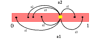
Let us go back to the updating of the belief state discussed earlier. Assume we start with a particular belief state b and we take action a1 and receive observation z1 after taking that action. Then our next belief state is fully determined. In fact, since we are assuming that there are a finite number of actions and a finite number of observations, given a belief state, there are a finite number of possible next belief states. These correspond to each combination of action and observation. The figure below shows this process graphically for a POMDP with two states (s1 and s2), two actions (a1 and a2) and three observations (z1, z2 and z3). The starting belief state is the big yellow dot and the resulting belief states are the smaller black dots. The arcs represent the process of transforming the belief state.

1D belief space for a 2 state POMDP

Note that this shows all possible resulting belief states. Since observations are probabilistic, each resulting belief state has a probability associated with it. More clearly stated: if we take an action and get an observation, then we know with certainty what our next belief state is. However, before we decide to take an action, each resulting belief state has a particular probability associated with it and there are as many possible next belief states as there are observations (for a given action). Note that for a given action, the next belief state probabilities must sum to 1. Also, it is possible that different action-observation combinations could lead to the same belief state, so there may be fewer next belief states than we first mentioned.

It turns out that the process of maintaining the belief state is Markovian; the next belief state depends only on the current belief state (and the current action and observation). In fact, we can convert a discrete POMDP problem into a continuous space CO-MDP problem where the continuous space is the belief space. The transitions of this new continuous space CO-MDP are easily derived from the transition and observation probabilities of the POMDP (remember: no formulas here). What this means is that we are now back to solving a CO-MDP and we can use the value iteration (VI) algorithm. However, we will need to adapt the algorithm some.

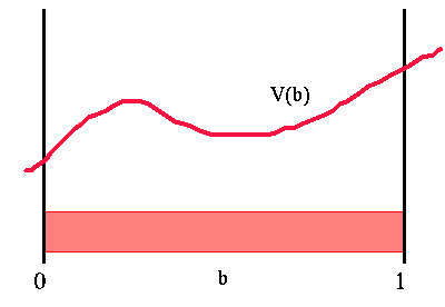
The big problem using value iteration here is the continuous state space. In CO-MDP value iteration we could simply maintain a table with one entry per state. The value of each state is stored in the table and we have a nice finite representation of the value function. Since we now have a continuous space, the value function could be some arbitrary function over belief space. The figure below shows a sample value function over belief space. Here 'b' is a belief space and the value function, 'V(b)', is a function of 'b'. Thus our first problem is how we can easily represent this value function.

Value function over belief space

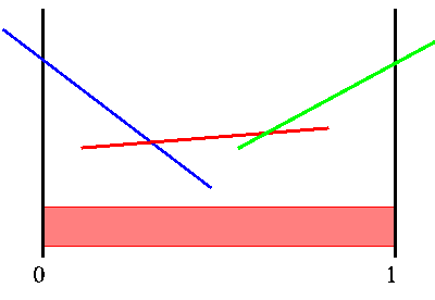
Fortunately, the POMDP formulation imposes some nice restrictions on the form of the solutions to the continuous space CO-MDP that is derived from the POMDP. The key insight is that the finite horizon value function is piecewise linear and convex (PWLC) for every horizon length. This means that for each iteration of value iteration, we only need to find a finite number of linear segments that make up the value function.

The figure below shows a sample value function over belief space for a POMDP. The vertical axis is the value, while the horizontal axis is the belief state. The POMDP value function is the upper surface of a finite number of linear segments. We have colored the segments for a reason to be explained later.

Sample PWLC value function

These linear segments will completely specify the value function (over belief space) that we desire. These amount to nothing more than lines or, more generally, hyper-planes through belief space. We can simply represent each hyper-plane with a vector of numbers, which are the coefficients of the equation of the hyper-plane. The value at any given belief state is found by plugging in the belief state into the hyper-planes equation. If we represent the hyper-plane as a vector (i.e., the equation coefficients) and each belief state as a vector (the probability at each state) then the value of a belief point is simply the dot product of the two vectors. (This is dangerously close to a formula, isn't it?)

We can now represent the value function for each horizon as a set of vectors. To find the value of a belief state, we simply find the vector that has the largest dot product with the belief state.

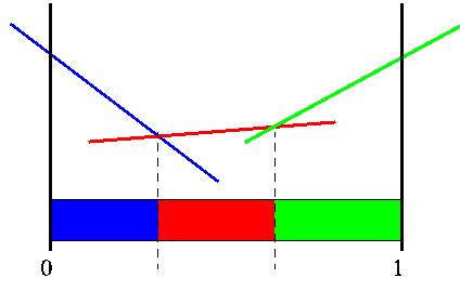
Instead of linear segments over belief space, another way to view the function is that it partitions belief space into a finite number of segments. We will be using both the value function and this partitioning representation to explain the algorithms. Keep in mind that they are more or less interchangeable.

Sample PWLC function and its partition of belief space

　　Now let's return to the value iteration algorithm. We have a continuous space CO-MDP and we were discussing adapting value iteration to this. The first problem we encountered was how to represent a value function over a continuous space. Since each horizon's value function is PWLC, we solved this problem, by representing the value function as a set of vectors (coefficients of the hyper-planes).

　　Unfortunately, the continuous space causes us further problems. In each iteration of value iteration in the discrete state space, we would find a state's new value by looping over all the possible next states. However, for continuous state CO-MDPs it is impossible to enumerate all possible states (can you say "uncountably infinite"?).

　　This is the main obstacle that needs to be overcome and the specific algorithms described later are all different approaches to solve this difficulty. Once we overcome this difficulty, the problem is solved and value iteration works the same here as in the discrete CO-MDP case. The problem now boils down to（可归结为） one stage of value iteration; given a set of vectors representing the value function for horizon 'h', we just need to generate the set of vectors for the value function of horizon 'h+1'