对于牛逼的程序员,人家都喜欢叫他大神;因为大神很牛逼,人家需要一个小时完成的技术问题,他就20分钟就搞定。Keras框架是一个高度集成的框架,学好它,就犹如掌握一个法宝,可以呼风唤雨。所以学keras 犹如在修仙,呵呵。请原谅我无厘头的逻辑。
ResNet
关于ResNet算法,在归纳卷积算法中有提到了,可以去看看。
1, ResNet 要解决的问题
ResNet要解决的问题是在求损失函数最小值时,梯度下降太快了,无法捕捉到最优解。
解决的方法是在求激活函数值 A值的时候
a^[l+1] =g(z^[l+1] +?)
〖?可以是a〗^([l-1]) 也可以是a^([l])等等
这样就能避免梯度下降过快
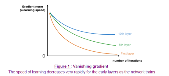
以上图是不同层数的模型的下降曲线
2, 构建自己的ResNet模型
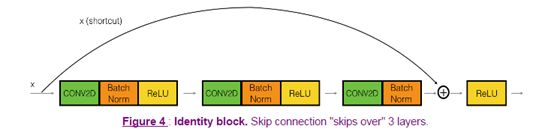
在resnet网络中,identity block的跳跃可能有1个或者2(conv2D+batchnorm+Relu)个,下面是两个可选图:
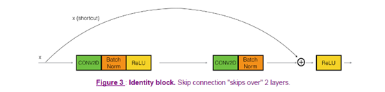
或者:
import numpy as np
import tensorflow as tf
from keras import layers
from keras.layers import Input, Add, Dense, Activation, ZeroPadding2D, BatchNormalization, Flatten, Conv2D, AveragePooling2D, MaxPooling2D, GlobalMaxPooling2D
from keras.models import Model, load_model
from keras.preprocessing import image
from keras.utils import layer_utils
from keras.utils.data_utils import get_file
from keras.applications.imagenet_utils import preprocess_input
import pydot
from IPython.display import SVG
from keras.utils.vis_utils import model_to_dot
from keras.utils import plot_model
from resnets_utils import *
from keras.initializers import glorot_uniform
import scipy.misc
from matplotlib.pyplot import imshow
%matplotlib inline

import keras.backend as K
K.set_image_data_format('channels_last')
K.set_learning_phase(1)
from keras.layers import Input, Add, Dense, Activation, ZeroPadding2D, BatchNormalization, Flatten, Conv2D, AveragePooling2D, MaxPooling2D, GlobalMaxPooling2D
from keras.models import Model, load_model
红色字体是重点关注的函数,很多在上节就已经说明,这里是BatchNormalization函数是为了规范化通道参数的,都必须给予命名:bn_name_base+’2?’
Activation 函数就不用命名了

2.1 创建标识块 identify block
def identity_block(X, f, filters, stage, block):
    """
    ##参数说明
   ## X:输入的维度 (m, n_H_prev, n_W_prev, n_C_prev)
   ## f:整数,中间conv2D的维度
   ##filters 过滤核的维度
   ## block 用于命名网络中的层
  ###返回值: 维度为(n_H, n_W, n_C)

   ###返回值: 维度为(n_H, n_W, n_C)
    """

    ##定义偏差
    conv_name_base = 'res' + str(stage) + block + '_branch'
    bn_name_base = 'bn' + str(stage) + block + '_branch'

    ##过滤核
    F1, F2, F3 = filters

    ##保存输入的值
    X_shortcut = X

    # #第一层卷积
    X = Conv2D(filters = F1, kernel_size = (1, 1), strides = (1,1), padding = 'valid', name = conv_name_base + '2a', kernel_initializer = glorot_uniform(seed=0))(X)
    X = BatchNormalization(axis = 3, name = bn_name_base + '2a')(X)
    X = Activation('relu')(X)

    ### START CODE HERE ###

    # Second component of main path (≈3 lines)
    X = Conv2D(filters = F2, kernel_size = (f, f), strides = (1,1), padding = 'same', name = conv_name_base + '2b', kernel_initializer = glorot_uniform(seed=0))(X)
    X = BatchNormalization(axis=3, name = bn_name_base + '2b')(X)
    X = Activation('relu')(X)

    # Third component of main path (≈2 lines)
    X = Conv2D(filters = F3, kernel_size = (1, 1), strides = (1,1), padding = 'valid', name = conv_name_base + '2c', kernel_initializer = glorot_uniform(seed=0))(X)
    X = BatchNormalization(axis=3, name = bn_name_base + '2c')(X)

    ###添加shortcut操作的激化
    X = layers.add([X, X_shortcut])
    X = Activation('relu')(X)

    ### END CODE HERE ###

    return X
小测:
tf.reset_default_graph()

with tf.Session() as test:
    np.random.seed(1)
    A_prev = tf.placeholder("float", [3, 4, 4, 6])
    X = np.random.randn(3, 4, 4, 6)
    A = identity_block(A_prev, f = 2, filters = [2, 4, 6], stage = 1, block = 'a')
    test.run(tf.global_variables_initializer())
    out = test.run([A], feed_dict={A_prev: X, K.learning_phase(): 0})
    print("out = " + str(out[0][1][1][0]))
结果:
out[ 0.94822985 0. 1.16101444 2.747859 0. 1.36677003]
2.2 卷积块 convolutional_block
卷积块主要是为了适配=g(+?)例子中?的维度跟的维度不匹配的现象,具体是在shortcut增加一个卷积,使其维度能都适配,而且是没有经过activation激活过的,如图:
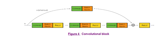
这样就可以通过卷积核的维度达到我们想到的维度减少非线性的函数操作。
def convolutional_block(X, f, filters, stage, block, s = 2):
    """
    参数跟identity_block是一样的,就多了一个
    s=2 表示卷积的步长
    """

    # defining name basis
    conv_name_base = 'res' + str(stage) + block + '_branch'
    bn_name_base = 'bn' + str(stage) + block + '_branch'

    # Retrieve Filters
    F1, F2, F3 = filters

    # Save the input value
    X_shortcut = X


    ##### MAIN PATH #####
    # First component of main path
    X = Conv2D(F1, (1, 1), strides = (s,s), name = conv_name_base + '2a', padding='valid', kernel_initializer = glorot_uniform(seed=0))(X)
    X = BatchNormalization(axis = 3, name = bn_name_base + '2a')(X)
    X = Activation('relu')(X)

    ### START CODE HERE ###

    # Second component of main path (≈3 lines)
    X = Conv2D(F2, (f, f), strides = (1, 1), name = conv_name_base + '2b',padding='same', kernel_initializer = glorot_uniform(seed=0))(X)
    X = BatchNormalization(axis = 3, name = bn_name_base + '2b')(X)
    X = Activation('relu')(X)

    # Third component of main path (≈2 lines)
    X = Conv2D(F3, (1, 1), strides = (1, 1), name = conv_name_base + '2c',padding='valid', kernel_initializer = glorot_uniform(seed=0))(X)
    X = BatchNormalization(axis = 3, name = bn_name_base + '2c')(X)

    ##### SHORTCUT PATH #### (≈2 lines)
    X_shortcut = Conv2D(F3, (1, 1), strides = (s, s), name = conv_name_base + '1',padding='valid', kernel_initializer = glorot_uniform(seed=0))(X_shortcut)
    X_shortcut = BatchNormalization(axis = 3, name = bn_name_base + '1')(X_shortcut)

    # Final step: Add shortcut value to main path, and pass it through a RELU activation (≈2 lines)
    X = layers.add([X, X_shortcut])
    X = Activation('relu')(X)

    ### END CODE HERE ###

    return X
小测:
tf.reset_defalut_graph()

with tf.Session() as test:
    np.random.seed(1)
    A_prev=tf.placeholder(“float”,[3,4,4,6])
    X=np.random.randn(3,4,4,6)
    A=convolutional_block(A_prev,f=2,filters=[2,4,6],stage=1,block=’a’)
    test.run(tf.global_variable_initializer())
    out.test.run([A],feed_dict={A_prev:X,K.learning_phase():0})
   print(“out=”+str(out[0][1][1][0]))
结果:
结果: out = [ 0.09018463 1.23489773 0.46822017 0.0367176 0. 0.65516603]
2.3 构建完整的例子
接下来我们根据
CONV2D -> BATCHNORM -> RELU -> MAXPOOL -> CONVBLOCK -> IDBLOCK*2 -> CONVBLOCK -> IDBLOCK*3
-> CONVBLOCK -> IDBLOCK*5 -> CONVBLOCK -> IDBLOCK*2 -> AVGPOOL -> TOPLAYER构建一个完整的resnet网络
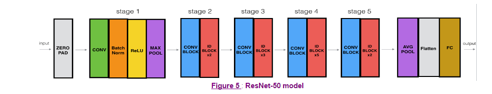
def ResNet50(input_shape = (64, 64, 3), classes = 6):
    """
    Implementation of the popular ResNet50 the following architecture:
    CONV2D -> BATCHNORM -> RELU -> MAXPOOL -> CONVBLOCK -> IDBLOCK*2 -> CONVBLOCK -> IDBLOCK*3
    -> CONVBLOCK -> IDBLOCK*5 -> CONVBLOCK -> IDBLOCK*2 -> AVGPOOL -> TOPLAYER

    Arguments:
    input_shape -- shape of the images of the dataset
    classes -- integer, number of classes

    Returns:
    model -- a Model() instance in Keras
    """

    # Define the input as a tensor with shape input_shape
    X_input = Input(input_shape)


    # Zero-Padding
    X = ZeroPadding2D((3, 3))(X_input)

    # Stage 1
    X = Conv2D(64, (7, 7), strides = (2, 2), name = 'conv1', kernel_initializer = glorot_uniform(seed=0))(X)
    X = BatchNormalization(axis = 3, name = 'bn_conv1')(X)
    X = Activation('relu')(X)
    X = MaxPooling2D((3, 3), strides=(2, 2))(X)

    # Stage 2
    X = convolutional_block(X, f = 3, filters = [64, 64, 256], stage = 2, block='a', s = 1)
    X = identity_block(X, 3, [64, 64, 256], stage=2, block='b')
    X = identity_block(X, 3, [64, 64, 256], stage=2, block='c')

    ### START CODE HERE ###

    # Stage 3 (≈4 lines)
    # The convolutional block uses three set of filters of size [128,128,512], "f" is 3, "s" is 2 and the block is "a".
    # The 3 identity blocks use three set of filters of size [128,128,512], "f" is 3 and the blocks are "b", "c" and "d".
    X = convolutional_block(X, f = 3, filters=[128,128,512], stage = 3, block='a', s = 2)
    X = identity_block(X, f = 3, filters=[128,128,512], stage= 3, block='b')
    X = identity_block(X, f = 3, filters=[128,128,512], stage= 3, block='c')
    X = identity_block(X, f = 3, filters=[128,128,512], stage= 3, block='d')

    # Stage 4 (≈6 lines)
    # The convolutional block uses three set of filters of size [256, 256, 1024], "f" is 3, "s" is 2 and the block is "a".
    # The 5 identity blocks use three set of filters of size [256, 256, 1024], "f" is 3 and the blocks are "b", "c", "d", "e" and "f".
    X = convolutional_block(X, f = 3, filters=[256, 256, 1024], block='a', stage=4, s = 2)
    X = identity_block(X, f = 3, filters=[256, 256, 1024], block='b', stage=4)
    X = identity_block(X, f = 3, filters=[256, 256, 1024], block='c', stage=4)
    X = identity_block(X, f = 3, filters=[256, 256, 1024], block='d', stage=4)
    X = identity_block(X, f = 3, filters=[256, 256, 1024], block='e', stage=4)
    X = identity_block(X, f = 3, filters=[256, 256, 1024], block='f', stage=4)

    # Stage 5 (≈3 lines)
    # The convolutional block uses three set of filters of size [512, 512, 2048], "f" is 3, "s" is 2 and the block is "a".
    # The 2 identity blocks use three set of filters of size [256, 256, 2048], "f" is 3 and the blocks are "b" and "c".
    X = convolutional_block(X, f = 3, filters=[512, 512, 2048], stage=5, block='a', s = 2)

    # filters should be [256, 256, 2048], but it fail to be graded. Use [512, 512, 2048] to pass the grading
    X = identity_block(X, f = 3, filters=[256, 256, 2048], stage=5, block='b')
    X = identity_block(X, f = 3, filters=[256, 256, 2048], stage=5, block='c')

    # AVGPOOL (≈1 line). Use "X = AveragePooling2D(...)(X)"
    # The 2D Average Pooling uses a window of shape (2,2) and its name is "avg_pool".平均值池化
    X = AveragePooling2D(pool_size=(2,2))(X)

    ### END CODE HERE ###

    # output layer
    X = Flatten()(X)
    X = Dense(classes, activation='softmax', name='fc' + str(classes), kernel_initializer = glorot_uniform(seed=0))(X)


    # Create model
    model = Model(inputs = X_input, outputs = X, name='ResNet50')

    return model
2.4 执行模型
1)加载模型
model = ResNet50(input_shape = (64, 64, 3), classes = 6)
2)编译模型
model.compile(optimizer='adam', loss='categorical_crossentropy', metrics=['accuracy'])
3)加载数据,训练模型
X_train_orig, Y_train_orig, X_test_orig, Y_test_orig, classes = load_dataset()

# Normalize image vectors
X_train = X_train_orig/255.
X_test = X_test_orig/255.

# Convert training and test labels to one hot matrices
Y_train = convert_to_one_hot(Y_train_orig, 6).T
Y_test = convert_to_one_hot(Y_test_orig, 6).T

print ("number of training examples = " + str(X_train.shape[0]))
print ("number of test examples = " + str(X_test.shape[0]))
print ("X_train shape: " + str(X_train.shape))
print ("Y_train shape: " + str(Y_train.shape))
print ("X_test shape: " + str(X_test.shape))
print ("Y_test shape: " + str(Y_test.shape))
model.fit(X_train, Y_train, epochs = 20, batch_size = 32)
4)测试模型
preds = model.evaluate(X_test, Y_test)
print ("Loss = " + str(preds[0]))
print ("Test Accuracy = " + str(preds[1]))
输出结果:
120/120 [==============================] - 9s 72ms/step
Loss = 0.729047638178
Test Accuracy = 0.891666666667
=========================================================
总结:这个例子到底位置,训练结果可能不是很满意,可以进一步加大测试集或者加大网络来达到优化的。
参考
中文keras手册:http://keras-cn.readthedocs.io/en/latest/layers/core_layer/
吴恩达网易课堂教程