机器学习（3）——梯度下降法

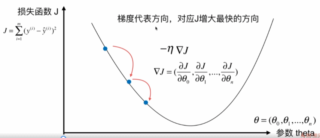
什么是梯度下降法

1. 不是一个机器学习算法
2. 是一种基于搜索的最优化方法
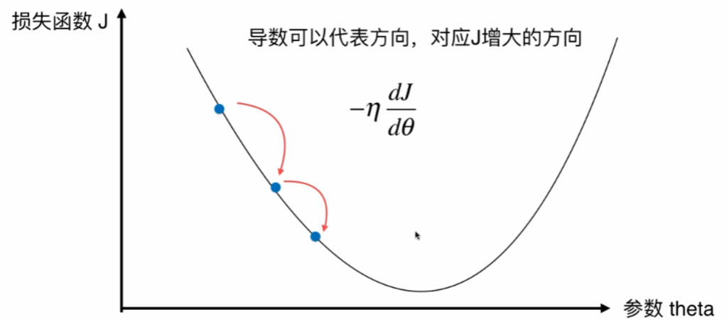
3. 作用：最小化一个损失函数
4. 梯度上升法：最大化一个效用函数

并不是所有函数都有唯一的极值点，解决方案：

1. 多次运行，随机化初始点
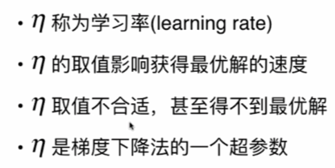
2. 梯度下降发的初始点也是一个超参数

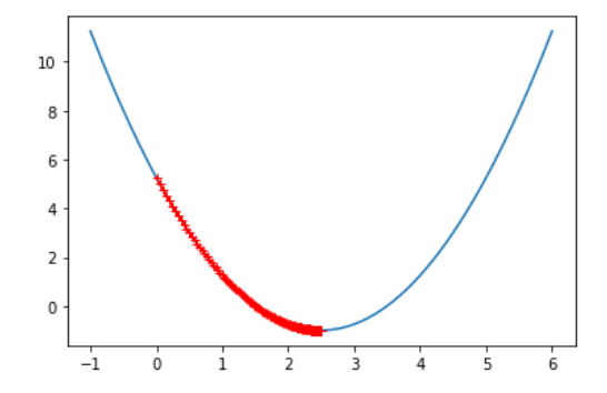
梯度下降法模拟

import numpy as np
import matplotlib.pyplot as plt

plot_x=np.linspace(-1,6,141)
plot_x

plot_y=(plot_x-2.5)**2-1

plt.plot(plot_x,plot_y)
plt.show()

def dJ(theta):#求导
    return 2*(theta-2.5)
    
def J(theta): #损失函数
    return (theta-2.5)**2-1
    
def gradient_descent(initial_theta,eta,n_iters=1e4,eps=1e-8):
    theta=initial_theta
    theta_history.append(initial_theta)
    i_iter=0
    
    while i_iter<n_iters:#最多进行n_iters次梯度下降
        gradient=dJ(theta)
        last_theta=theta
        theta=theta-eta*gradient
        theta_history.append(theta)
        
        if(abs(J(theta)-J(last_theta))<eps):
            break
        i_iter+=1
    
def plot_theta_history():
    plt.plot(plot_x,plot_y)
    plt.plot(theta_history,J(np.array(theta_history)),color="r",marker="+")
    plt.show()
    
eta=0.01
theta_history=[]
gradient_descent(0,eta)
plot_theta_history()

因为学习率eta过高时，可能会出现无穷大-无穷大的情况，这在python里答案是nan，所以我们要对J()异常处理：

def J(theta):
    try:
        return (theta-2.5)**2-1.
    except:
        return float('inf')

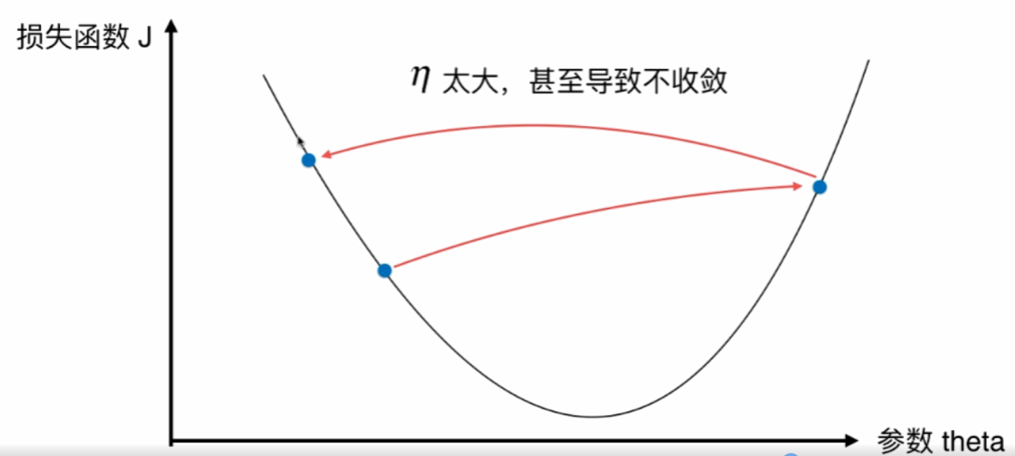
试一下eta=1.1：

eta=1.1
theta_history=[]
gradient_descent(0,eta)

theta_history[-1]

可以发现最后一个数是nan

迭代次数取少点，绘制一下图形：

eta=1.1
theta_history=[]
gradient_descent(0,eta,n_iters=10)
plot_theta_history()

线性回归中的梯度下降法

import numpy as np
import matplotlib.pyplot as plt

np.random.seed=666
x=2*np.random.random(size=100) #[0,2]的均匀分布
y=x*3.+4.+np.random.normal(size=100) #默认是列向量

X=x.reshape(-1,1)

plt.scatter(x,y)
plt.show()

def J(theta,X_b,y):
    try:
        return np.sum((y-X_b.dot(theta))**2)/len(X_b)
    except:
        return float('inf')
        
def dJ(theta,X_b,y):
    res=np.empty(len(theta))
    res[0]=np.sum(X_b.dot(theta)-y)
    for i in range(1,len(theta)):
        res[i]=(X_b.dot(theta)-y).dot(X_b[:,i])#可以看成先求前面的∑部分，最后再和X的第i列点积
    return res*2/len(X_b)  
    
def gradient_descent(X_b,y,initial_theta,eta,n_iters=1e4,eps=1e-8):
    theta=initial_theta
    i_iter=0
    
    while i_iter<n_iters:#最多进行n_iters次梯度下降
        gradient=dJ(theta,X_b,y)
        last_theta=theta
        theta=theta-eta*gradient
        
        if(abs(J(theta,X_b,y)-J(last_theta,X_b,y))<eps):
            break
        i_iter+=1
    return theta
    
X_b=np.hstack([np.ones((len(X),1)),X])
initial_theta=np.zeros(X_b.shape[1]) #和X的特征个数相同
eta=0.01

theta=gradient_descent(X_b,y,initial_theta,eta)

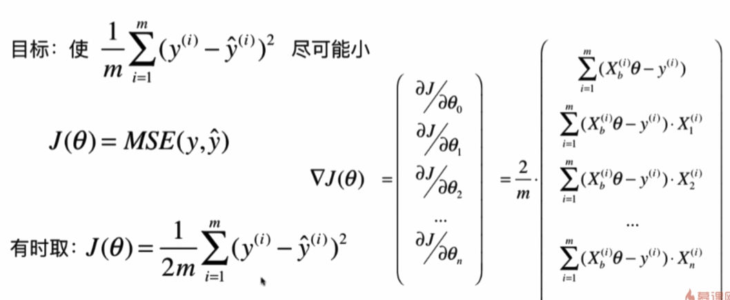
向量化

上面求到后的式子可以化成矩阵相乘：

图中右下角为最终答案，这是因为Xb是m（样本数）行n（特征值数）列的，所以Xb*theta是m行1列的，即列向量，python中默认是列向量，所以y也是列向量，那么Xb * theta - y要转置一下才能变成图中第一行的行向量，最后计算结果还要转置一下才能变成列向量。

添加了梯度下降训练的LinearRegression类：

import numpy as np
from sklearn.metrics import r2_score


class LinearRegression:

    def __init__(self):
        """初始化Linear Regression模型"""
        self.coef_ = None
        self.intercept_ = None
        self._theta = None

    def fit_normal(self, X_train, y_train):
        """根据训练数据集X_train, y_train训练Linear Regression模型"""
        assert X_train.shape[0] == y_train.shape[0], 
            "the size of X_train must be equal to the size of y_train"

        X_b = np.hstack([np.ones((len(X_train), 1)), X_train])
        self._theta = np.linalg.inv(X_b.T.dot(X_b)).dot(X_b.T).dot(y_train)

        self.intercept_ = self._theta[0]
        self.coef_ = self._theta[1:]

        return self

    def fit_gd(self, X_train, y_train, eta=0.01, n_iters=1e4):
        """根据训练数据集X_train, y_train, 使用梯度下降法训练Linear Regression模型"""
        assert X_train.shape[0] == y_train.shape[0], 
            "the size of X_train must be equal to the size of y_train"

        def J(theta, X_b, y):
            try:
                return np.sum((y - X_b.dot(theta)) ** 2) / len(y)
            except:
                return float('inf')

        def dJ(theta, X_b, y):
            return X_b.T.dot(X_b.dot(theta) - y) * 2. / len(y)

        def gradient_descent(X_b, y, initial_theta, eta, n_iters=1e4, epsilon=1e-8):

            theta = initial_theta
            cur_iter = 0

            while cur_iter < n_iters:
                gradient = dJ(theta, X_b, y)
                last_theta = theta
                theta = theta - eta * gradient
                if (abs(J(theta, X_b, y) - J(last_theta, X_b, y)) < epsilon):
                    break

                cur_iter += 1

            return theta

        X_b = np.hstack([np.ones((len(X_train), 1)), X_train])
        initial_theta = np.zeros(X_b.shape[1])
        self._theta = gradient_descent(X_b, y_train, initial_theta, eta, n_iters)

        self.intercept_ = self._theta[0]
        self.coef_ = self._theta[1:]

        return self

    def predict(self, X_predict):
        """给定待预测数据集X_predict，返回表示X_predict的结果向量"""
        assert self.intercept_ is not None and self.coef_ is not None, 
            "must fit before predict!"
        assert X_predict.shape[1] == len(self.coef_), 
            "the feature number of X_predict must be equal to X_train"

        X_b = np.hstack([np.ones((len(X_predict), 1)), X_predict])
        return X_b.dot(self._theta)

    def score(self, X_test, y_test):
        """根据测试数据集 X_test 和 y_test 确定当前模型的准确度"""

        y_predict = self.predict(X_test)
        return r2_score(y_test, y_predict)

    def __repr__(self):
        return "LinearRegression()"

import numpy as np
from sklearn import datasets

boston=datasets.load_boston()
X=boston.data
y=boston.target
X=X[y<50.0]
y=y[y<50.0]

from sklearn.model_selection import train_test_split
X_train,X_test,y_train,y_test=train_test_split(X,y,random_state=666,test_size=0.2)

%run f:python3玩转机器学习线性回归LinearRegression.py

lin_reg1=LinearRegression()
%time lin_reg1.fit_normal(X_train,y_train)
lin_reg1.score(X_test,y_test)

# 梯度下降法
lin_reg2=LinearRegression()
lin_reg2.fit_gd(X_train,y_train)

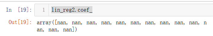
lin_reg2.coef_

X_train[:10,:]

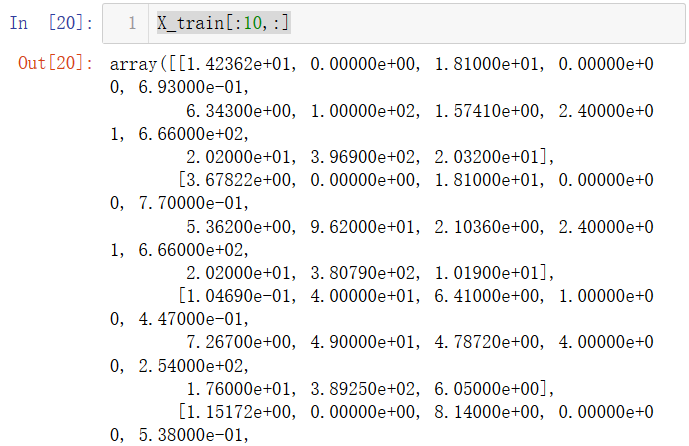
发现系数都是无穷大，说明学习率太大、训练数据数量级差距太大，导致梯度下降不收敛。

lin_reg2.fit_gd(X_train,y_train,eta=0.000001)

lin_reg2.score(X_test,y_test)#循环次数不够

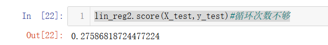
发现正确率很低，说明可能循环次数不够

%time lin_reg2.fit_gd(X_train,y_train,eta=0.000001,n_iters=1e6)

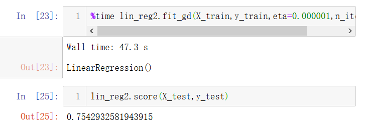
发现准确率提高了，但太耗时了，得另辟蹊径。

归一化

线性回归类中fit_normal采用的是求解正规方程，不涉及搜索的过程，所以不需要数据归一化，时间复杂度O（n^3）。

使用梯度下降法前，最好进行数据归一化。

from sklearn.preprocessing import StandardScaler

standardScaler=StandardScaler()
standardScaler.fit(X_train)

X_train_standard=standardScaler.transform(X_train)

lin_reg3=LinearRegression()
%time lin_reg3.fit_gd(X_train_standard,y_train)

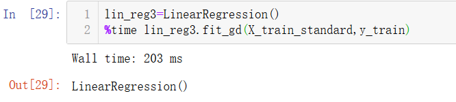
可以发现归一化后训练时间优化了很多。

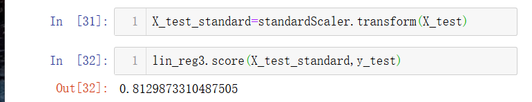
正确率也和正规方程一致了。

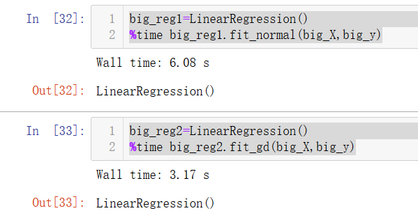
当然，我们可能会发现梯度下降居然比正规方程还慢一点。但是矩阵越大，梯度下降的优势就越强。

m=1000
n=5000
big_X=np.random.normal(size=(m,n)) #正态分布
true_theta=np.random.uniform(0.0,100.0,size=n+1) #n+1个[0,100]的数
big_y=big_X.dot(true_theta[1:])+true_theta[0]+np.random.normal(0.,10.,size=m) #加个均值为0，标准差为10的噪音

big_reg1=LinearRegression()
%time big_reg1.fit_normal(big_X,big_y)

big_reg2=LinearRegression()
%time big_reg2.fit_gd(big_X,big_y)

随机梯度下降法

用精度换时间消耗。

每次随机取一个样本i。

根据模拟退火的思想，学习率要随着迭代次数增加渐渐变小，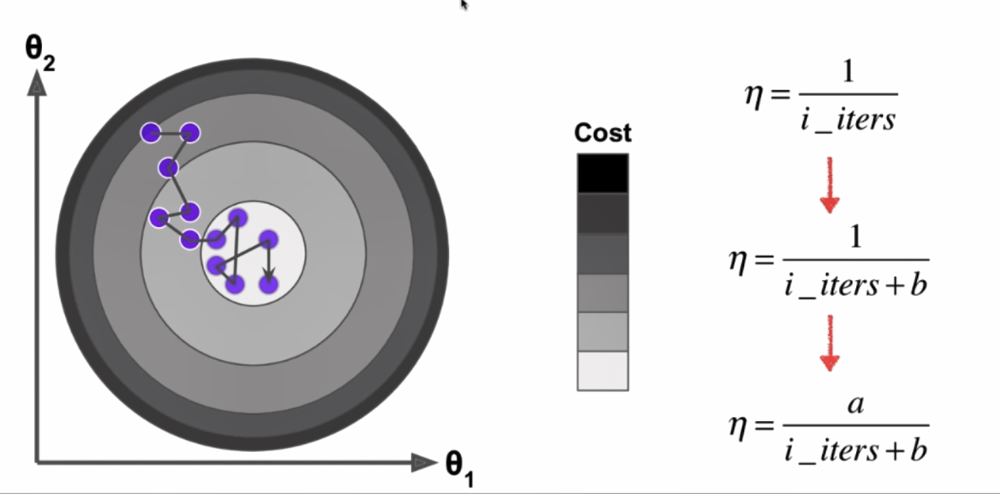

来个例子实战一下看看威力！

import numpy as np
import matplotlib.pyplot as plt

m=500000
x=np.random.normal(size=m) #列向量
X=x.reshape(-1,1)
y=4.*x+3.+np.random.normal(0,3,size=m) #加上噪音

def J(theta,X_b,y):
    try:
        return np.sum((y-X_b.dot(theta))**2)/len(y)
    except:
        return float('inf')

批量梯度下降：

def dJ(theta,X_b,y):
    return X_b.T.dot(X_b.dot(theta)-y)*2/len(y)
    
def gradient_descent(X_b,y,initial_theta,eta,n_iters=1e4,eps=1e-8):
    theta=initial_theta
    cur_iter=0
    
    while cur_iter < n_iters:
        gradient=dJ(theta,X_b,y)
        last_theta=theta
        theta=theta-eta*gradient
        if(abs(J(theta,X_b,y)-J(last_theta,X_b,y))<eps):
            break
        cur_iter+=1
    return theta
    
%%time
X_b=np.hstack([np.ones((len(x),1)),X])
initial_theta=np.zeros(X_b.shape[1])
eta=0.01
theta=gradient_descent(X_b,y,initial_theta,eta)

可以看出和我们刚开始设的斜率和截距是差不多的（4，3）

再看看随机梯度下降法：

def dJ_sgd(theta,X_b_i,y_i):
    return X_b_i.T.dot(X_b_i.dot(theta)-y_i)*2.
    
def sgd(X_b,y,initial_theta,n_iters):
    t0=1
    t1=50
    def learning_rate(t):
        return t0/(t+t1)
    theta=initial_theta
    for cur_iter in range(n_iters):
        rand_i=np.random.randint(len(X_b))
        gradient=dJ_sgd(theta,X_b[rand_i],y[rand_i])
        theta=theta-learning_rate(cur_iter)*gradient
    return theta
    
%%time
X_b=np.hstack([np.ones((len(X),1)),X])
initial_theta=np.zeros(X_b.shape[1])
theta=sgd(X_b,y,initial_theta,n_iters=len(X_b)//3) #这里把迭代次数设小一点以看随机梯度下降的威力

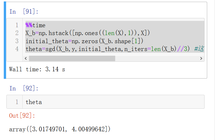
可以看出随机梯度下降法的速度快，准确率也不差！

添加了随机梯度下降训练的LinearRegression类：

import numpy as np


from sklearn.metrics import r2_score

class LinearRegression:

    def __init__(self):
        """初始化Linear Regression模型"""
        self.coef_ = None
        self.intercept_ = None
        self._theta = None

    def fit_normal(self, X_train, y_train):
        """根据训练数据集X_train, y_train训练Linear Regression模型"""
        assert X_train.shape[0] == y_train.shape[0], 
            "the size of X_train must be equal to the size of y_train"

        X_b = np.hstack([np.ones((len(X_train), 1)), X_train])
        self._theta = np.linalg.inv(X_b.T.dot(X_b)).dot(X_b.T).dot(y_train)

        self.intercept_ = self._theta[0]
        self.coef_ = self._theta[1:]

        return self

    def fit_bgd(self, X_train, y_train, eta=0.01, n_iters=1e4):
        """根据训练数据集X_train, y_train, 使用梯度下降法训练Linear Regression模型"""
        assert X_train.shape[0] == y_train.shape[0], 
            "the size of X_train must be equal to the size of y_train"

        def J(theta, X_b, y):
            try:
                return np.sum((y - X_b.dot(theta)) ** 2) / len(y)
            except:
                return float('inf')

        def dJ(theta, X_b, y):
            return X_b.T.dot(X_b.dot(theta) - y) * 2. / len(y)

        def gradient_descent(X_b, y, initial_theta, eta, n_iters=1e4, epsilon=1e-8):

            theta = initial_theta
            cur_iter = 0

            while cur_iter < n_iters:
                gradient = dJ(theta, X_b, y)
                last_theta = theta
                theta = theta - eta * gradient
                if (abs(J(theta, X_b, y) - J(last_theta, X_b, y)) < epsilon):
                    break

                cur_iter += 1

            return theta

        X_b = np.hstack([np.ones((len(X_train), 1)), X_train])
        initial_theta = np.zeros(X_b.shape[1])
        self._theta = gradient_descent(X_b, y_train, initial_theta, eta, n_iters)

        self.intercept_ = self._theta[0]
        self.coef_ = self._theta[1:]

        return self

    def fit_sgd(self, X_train, y_train, n_iters=50, t0=5, t1=50):
        # 此处的n_iters表示整个样本看几次
        """根据训练数据集X_train, y_train, 使用梯度下降法训练Linear Regression模型"""
        assert X_train.shape[0] == y_train.shape[0], 
            "the size of X_train must be equal to the size of y_train"
        assert n_iters >= 1

        def dJ_sgd(theta, X_b_i, y_i):
            return X_b_i * (X_b_i.dot(theta) - y_i) * 2.

        def sgd(X_b, y, initial_theta, n_iters=5, t0=5, t1=50):

            def learning_rate(t):
                return t0 / (t + t1)

            theta = initial_theta
            m = len(X_b)
            #以下代码保证每个样本都被遍历n_iters次
            for i_iter in range(n_iters):
                indexes = np.random.permutation(m)
                X_b_new = X_b[indexes,:]
                y_new = y[indexes]
                for i in range(m):
                    gradient = dJ_sgd(theta, X_b_new[i], y_new[i])
                    theta = theta - learning_rate(i_iter * m + i) * gradient

            return theta

        X_b = np.hstack([np.ones((len(X_train), 1)), X_train])
        initial_theta = np.random.randn(X_b.shape[1])
        self._theta = sgd(X_b, y_train, initial_theta, n_iters, t0, t1)

        self.intercept_ = self._theta[0]
        self.coef_ = self._theta[1:]

        return self

    def predict(self, X_predict):
        """给定待预测数据集X_predict，返回表示X_predict的结果向量"""
        assert self.intercept_ is not None and self.coef_ is not None, 
            "must fit before predict!"
        assert X_predict.shape[1] == len(self.coef_), 
            "the feature number of X_predict must be equal to X_train"

        X_b = np.hstack([np.ones((len(X_predict), 1)), X_predict])
        return X_b.dot(self._theta)

    def score(self, X_test, y_test):
        """根据测试数据集 X_test 和 y_test 确定当前模型的准确度"""

        y_predict = self.predict(X_test)
        return r2_score(y_test, y_predict)

    def __repr__(self):
        return "LinearRegression()"

再用波士顿房价的例子测试一下：

import numpy as np
from sklearn import datasets
from sklearn.model_selection import train_test_split
boston=datasets.load_boston()
X=boston.data
y=boston.target
X=X[y<50.0]
y=y[y<50.0]
X_train,X_test,y_train,y_test=train_test_split(X,y,random_state=666,test_size=0.2)

from sklearn.preprocessing import StandardScaler

standardScaler=StandardScaler()
standardScaler.fit(X_train)
X_train_standard=standardScaler.transform(X_train)
X_test_standard=standardScaler.transform(X_test)

%run f:python3玩转机器学习线性回归LinearRegression.py

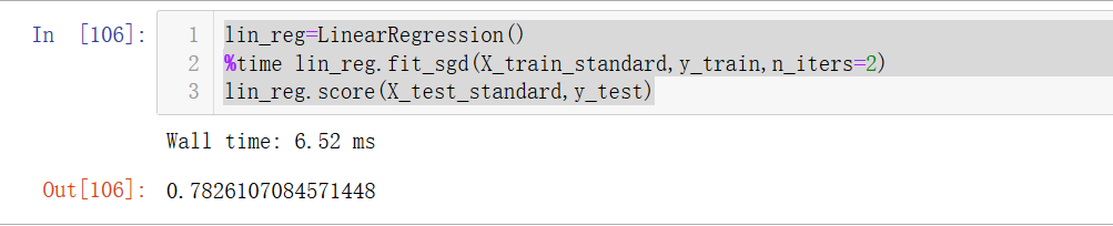
lin_reg=LinearRegression()
%time lin_reg.fit_sgd(X_train_standard,y_train,n_iters=2)
lin_reg.score(X_test_standard,y_test)

发现准确率和0.81差不多了：

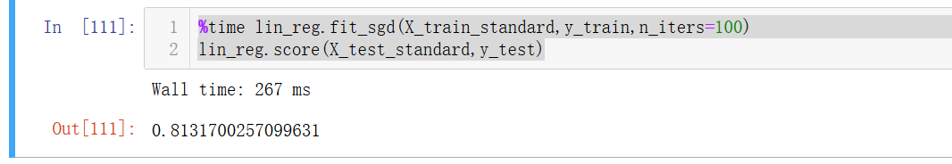
迭代次数调大：

%time lin_reg.fit_sgd(X_train_standard,y_train,n_iters=100)
lin_reg.score(X_test_standard,y_test)

scikit-learn中的随机梯度下降：

from sklearn.linear_model import SGDRegressor

sgd_reg=SGDRegressor()
%time sgd_reg.fit(X_train_standard,y_train)
sgd_reg.score(X_test_standard,y_test)

sgd_reg=SGDRegressor(max_iter=100)
%time sgd_reg.fit(X_train_standard,y_train)
sgd_reg.score(X_test_standard,y_test)

关于梯度的调试

有时候可能梯度求错了但不会报错，这就很坑。

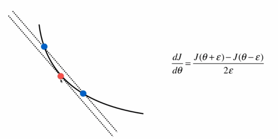
取相邻两个点，这两点的斜率（纵坐标之差/横坐标之差）和切线斜率是差不多的。

对每一个tehta求一遍theta+和theta-，再根据右下角的式子就可以算出这一点切线的斜率，但这样做是非常耗时间的，因此这种方法只适合调试用。

import numpy as np
import matplotlib.pyplot as plt

 np.random.seed=666
 X=np.random.random(size=(1000,10))
 true_theta = np.arange(1,12,dtype=float)
X_b=np.hstack([np.ones((len(X),1)),X])
y=X_b.dot(true_theta)+np.random.normal(size=1000) #加上噪音

def J(theta,X_b,y):
    try:
        return np.sum((y-X_b.dot(theta))**2)/len(X_b)
    except:
        return float('inf')
        
def dJ_math(theta,X_b,y):#数学推导求导
    return X_b.T.dot(X_b.dot(theta)-y)*2./len(y)
    
def dJ_debug(theta,X_b,y,epsilon=0.01):#调试求导
    res=np.empty(len(theta))
    for i in range(len(theta)):
        theta_1=theta.copy()
        theta_1[i]+=epsilon
        theta_2=theta.copy()
        theta_2[i]-=epsilon
        res[i]=(J(theta_1,X_b,y)-J(theta_2,X_b,y))/(2*epsilon)
    return res
    
def gradient_descent(dJ,X_b,y,initial_theta,eta,n_iters=1e4,eps=1e-8):#传入求导方法
    theta=initial_theta
    cur_iter=0
    while cur_iter < n_iters:
        gradient=dJ(theta,X_b,y)
        last_theta=theta
        theta=theta-eta*gradient
        if(abs(J(theta,X_b,y)-J(last_theta,X_b,y))<eps):
            break
        cur_iter+=1
    return theta
    
X_b=np.hstack([np.ones((len(X),1)),X])
initial_theta=np.zeros(X_b.shape[1])
eta=0.01
%time theta=gradient_descent(dJ_debug,X_b,y,initial_theta,eta)
theta

%time theta=gradient_descent(dJ_math,X_b,y,initial_theta,eta)
theta

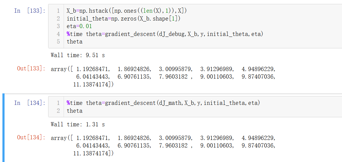
验证出我们数学推导的求导是正确的。

可以发现调试法求导只用到了J()，所以使用所有的损失函数的，而数学推导求导是根据J（）来推导出来的。

有关梯度下降的深入讨论

随机：

1. 跳出局部最优解，更容易找到全局最优解
2. 更快的运行速度
3. 机器学习领域很多算法都要使用随机的特点：随机搜索、随机森林

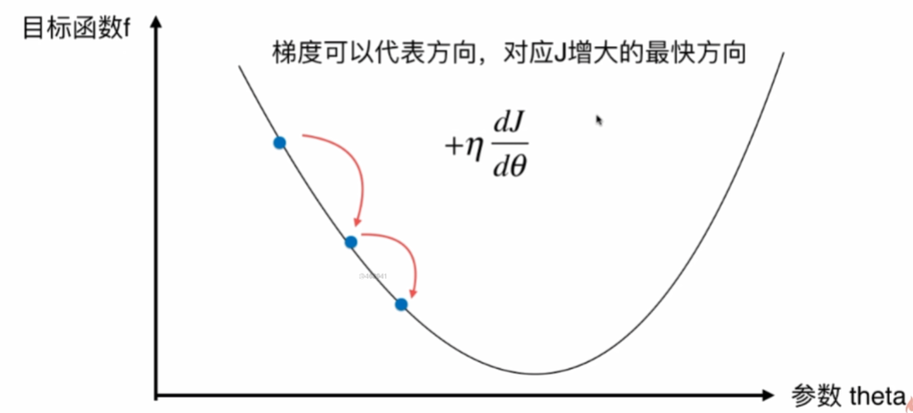
求损失函数J的最大值，可以用梯度上升法：