机器学习-支持向量机理论与应用(线性可分)

1. 背景：

     1.1 最早是由 Vladimir N. Vapnik 和 Alexey Ya. Chervonenkis 在1963年提出

     1.2 目前的版本(soft margin)是由Corinna Cortes 和 Vapnik在1993年提出，并在1995年发表

     1.3 深度学习（2012）出现之前，SVM被认为机器学习中近十几年来最成功，表现最好的算法

 

2. 机器学习的一般框架：

     训练集 => 提取特征向量 => 结合一定的算法（分类器：比如决策树，KNN）=>得到结果

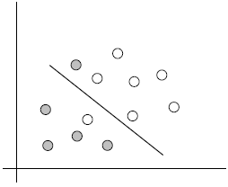
3. 介绍：

          

     3.1 例子：

     

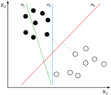
       两类？哪条线最好？

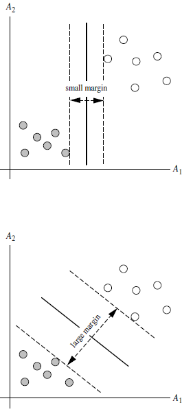
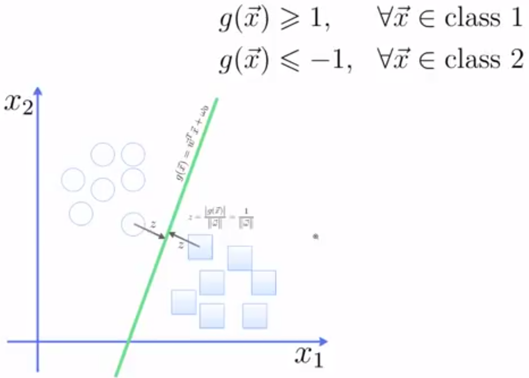
     3.2 SVM寻找区分两类的超平面（hyper plane), 使边际(margin)最大

         

          总共可以有多少个可能的超平面？无数条

          如何选取使边际(margin)最大的超平面 (Max Margin Hyperplane)？

          超平面到一侧最近点的距离等于到另一侧最近点的距离，两侧的两个超平面平行

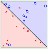
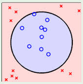
    3.3. 线性可区分(linear separable) 和 线性不可区分 （linear inseparable) 

          

          

 

       

4. 定义与公式建立

 

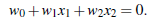
          超平面可以定义为：

　　　　　　　　　　

          W: weight vector,   

　　　　　　　      　  

　　   n :是特征值的个数

          X: 训练实例

          b: bias

         

     4.1 假设2维特征向量：X = (x₁, X₂)

           把 b 想象为额外的 wight

           超平面方程变为：

　　　　　　　　

           所有超平面右上方的点满足：

　　　　　　　　　　　

           所有超平面左下方的点满足：

　　　　　　　　 

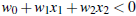
              调整weight，使超平面定义边际的两边：

　　　　　　　　

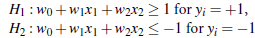
           综合以上两式，得到：

　　　　　　　　  

             所有坐落在边际两边的超平面上的点被称作”支持向量(support vectors)"

 　　     分界的超平面和H1或H2上任意一点的距离为 

                                       

           (其中||W||是向量的范数(norm))

                                       

              所以，最大边际距离为：

                                       

5. 求解

 

     5.1  SVM如何找出最大边际的超平面呢(MMH)？

                           

            利用一些数学推倒，以上公式 （1）可变为有限制的凸优化问题(convex quadratic optimization)

            利用 Karush-Kuhn-Tucker (KKT)条件和拉格朗日公式，可以推出MMH可以被表示为以下“决定边 界(decision boundary)”                                                                     

                                                  

            其中，

                                      

            是支持向量点 

　　　　　　　　　　
            (support vector)的类别标记（class label)                                   

                                     
　　     是要测试的实例

                                         

            都是单一数值型参数，由以上提到的最有算法得出           

                                     
　　     是支持向量点的个数

 

     5.2  对于任何测试（要归类的）实例，带入以上公式，得出的符号是正还是负决定

 

6. 实例一：

 

 

 

 

 

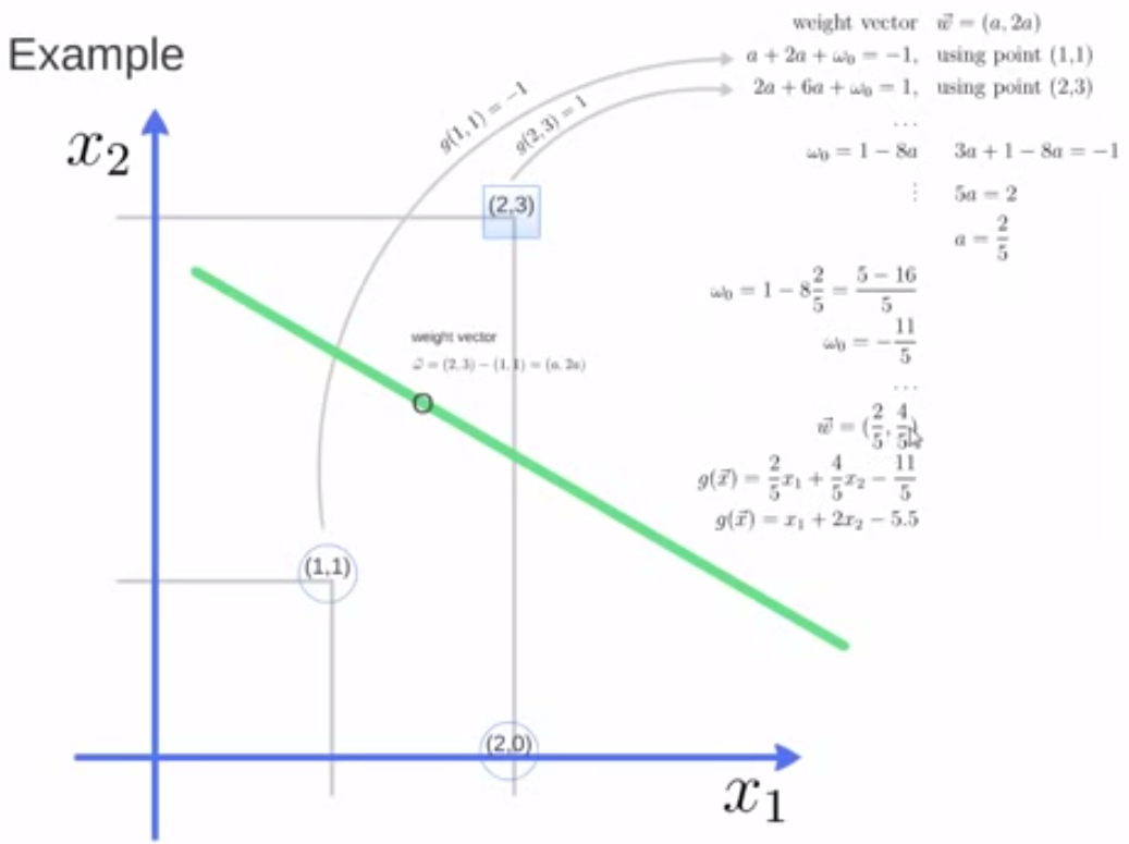
 调用Python中库函数实现

# -*- coding:utf-8 -*-

from sklearn import svm

x = [[2,0],[1,1],[2,3]]
#python中的两类问题分类标签
y = [0,0,1]

clf = svm.SVC(kernel='linear')
clf.fit(x,y)

print(clf)

#get support vectors 支持向量
print(clf.support_vectors_)

#get index of support vectors 支持向量的下标
print(clf.support_)

#get number of support vectors for each class
print(clf.n_support_)

　　结果

SVC(C=1.0, cache_size=200, class_weight=None, coef0=0.0,
  decision_function_shape=None, degree=3, gamma='auto', kernel='linear',
  max_iter=-1, probability=False, random_state=None, shrinking=True,
  tol=0.001, verbose=False)
[[ 1.  1.]
 [ 2.  3.]]
[1 2]
[1 1]

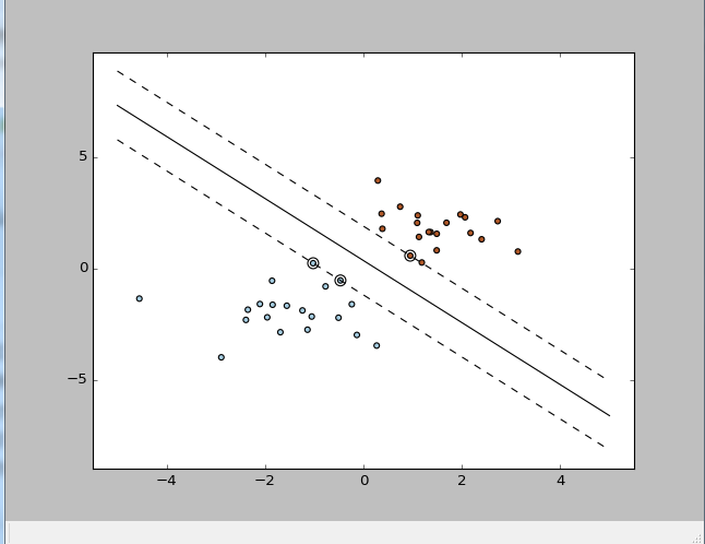
7.实例二

# -*- coding:utf-8 -*-

import numpy as np
import pylab as pl
from sklearn import  svm

#we create 40 separable points
np.random.seed(0)#控制每次的数据相同
#- [2,2] + [2,2] 是为了使得两组正态分布的数据呈线性上下分开
X = np.r_[np.random.randn(20,2) - [2,2], np.random.randn(20,2) + [2,2]]
Y = [0]*20 + [1]*20 #类标签

#fit the model
clf = svm.SVC(kernel='linear')
clf.fit(X ,Y)

#get the separating hyperplane
w = clf.coef_[0]
a = -w[0] / w[1] #斜率
xx = np.linspace(-5,5) #[-5,-4,-3,...,5]
#clf.intercept_[0]) 为w[3]
yy = a * xx - (clf.intercept_[0]) / w[1]

# plot the parallels to the separating hyperplane that pass through the support vectors
b = clf.support_vectors_[0]#取出第一个支持向量
yy_down = a * xx + (b[1] - a*b[0]) #(b[1] - a*b[0])下面直线的截距
b = clf.support_vectors_[-1]#最后一个支持向量
yy_up = a * xx + (b[1] - a*b[0])

print("w: ", w)
print("a: ", a)

# print "xx: ", xx
# print "yy: ", yy
print("support_vectors_: ", clf.support_vectors_)
print("clf.coef_: ", clf.coef_)

# switching to the generic n-dimensional parameterization of the hyperplan to the 2D-specific equation
# of a line y=a.x +b: the generic w_0x + w_1y +w_3=0 can be rewritten y = -(w_0/w_1) x + (w_3/w_1)


# plot the line, the points, and the nearest vectors to the plane
pl.plot(xx, yy, 'k-')
pl.plot(xx, yy_down, 'k--')
pl.plot(xx, yy_up, 'k--')

pl.scatter(clf.support_vectors_[:, 0], clf.support_vectors_[:, 1],
          s=80, facecolors='none')
pl.scatter(X[:, 0], X[:, 1], c=Y, cmap=pl.cm.Paired)

pl.axis('tight')
pl.show()

　　结果

w:  [ 0.90230696  0.64821811]
a:  -1.39198047626
support_vectors_:  [[-1.02126202  0.2408932 ]
 [-0.46722079 -0.53064123]
 [ 0.95144703  0.57998206]]
clf.coef_:  [[ 0.90230696  0.64821811]]