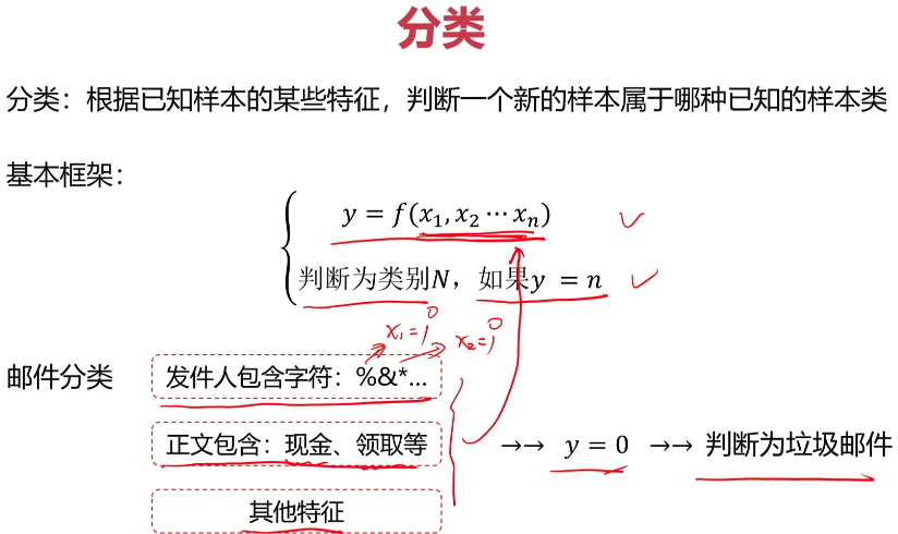
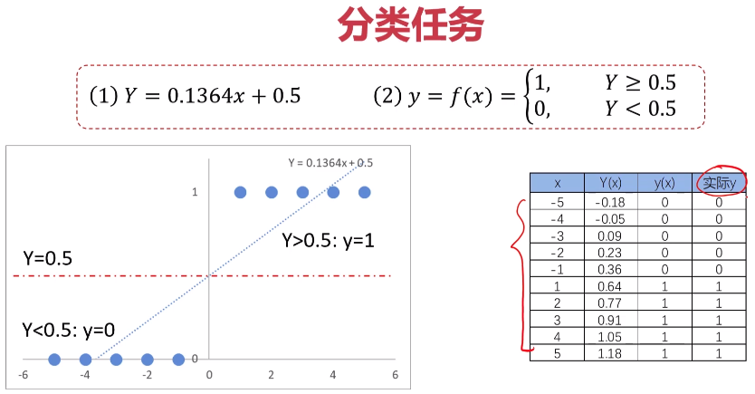
- 分类问题介绍


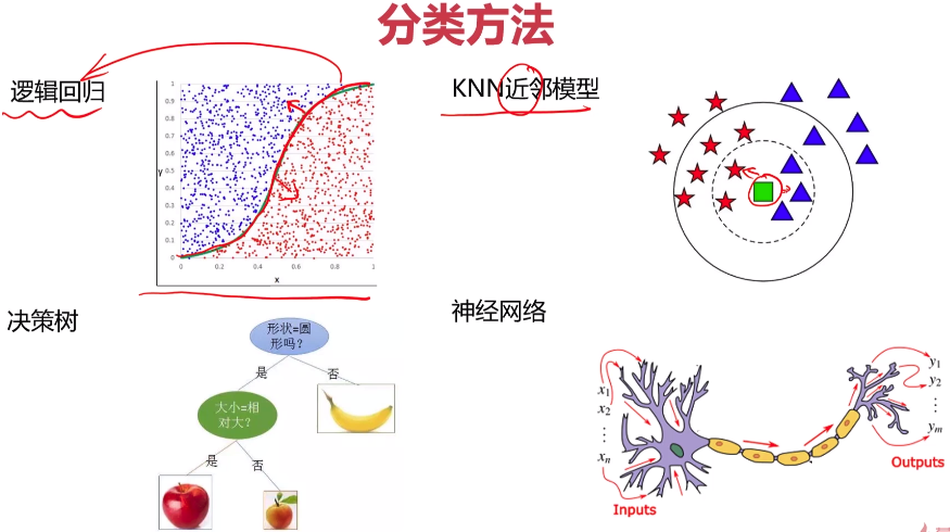


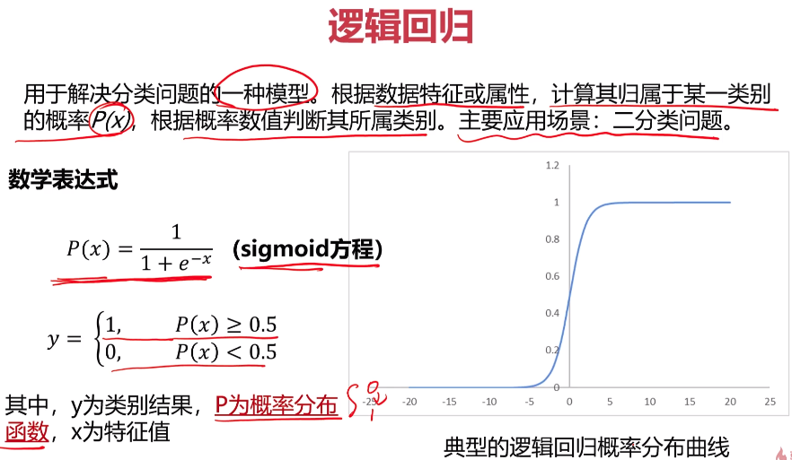
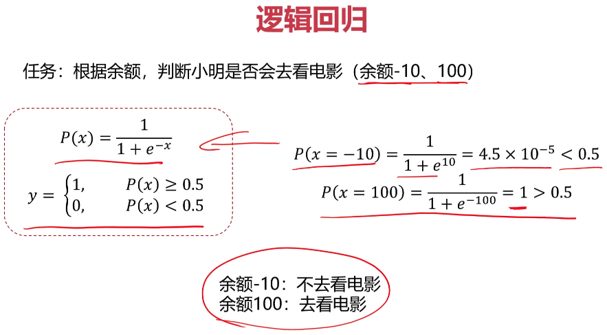
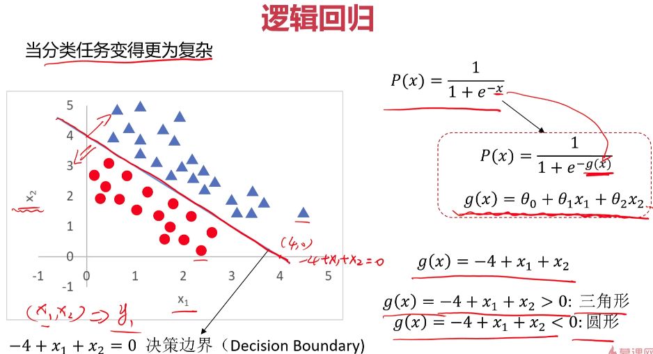
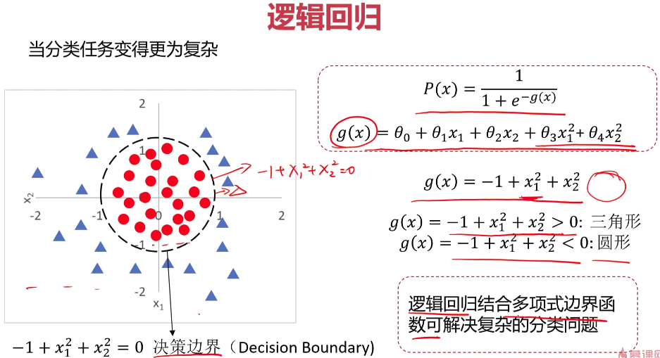
- 逻辑回归


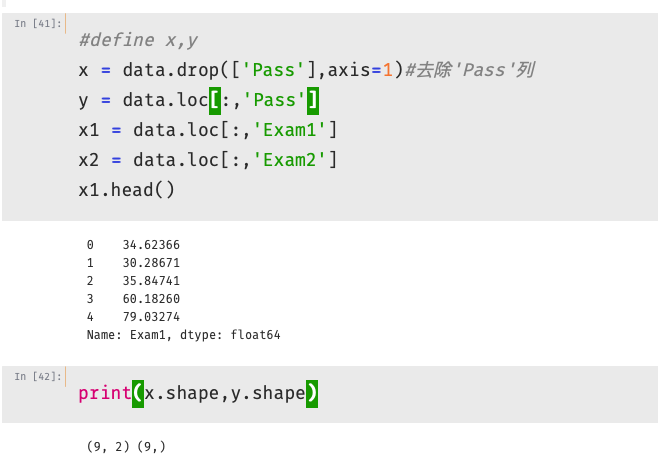
- 实战准备


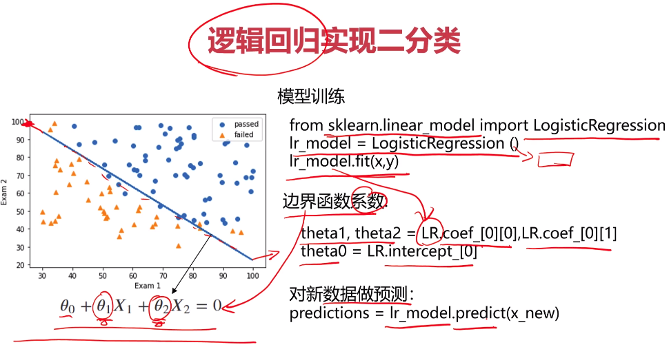

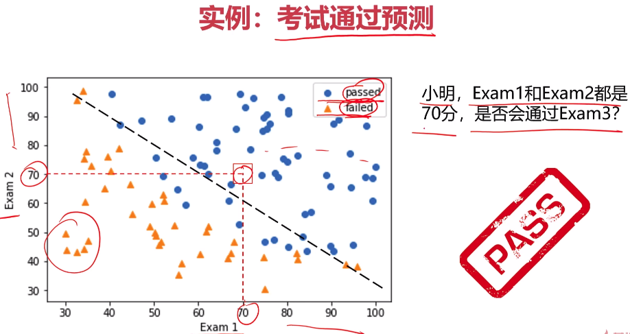
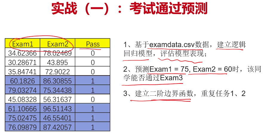
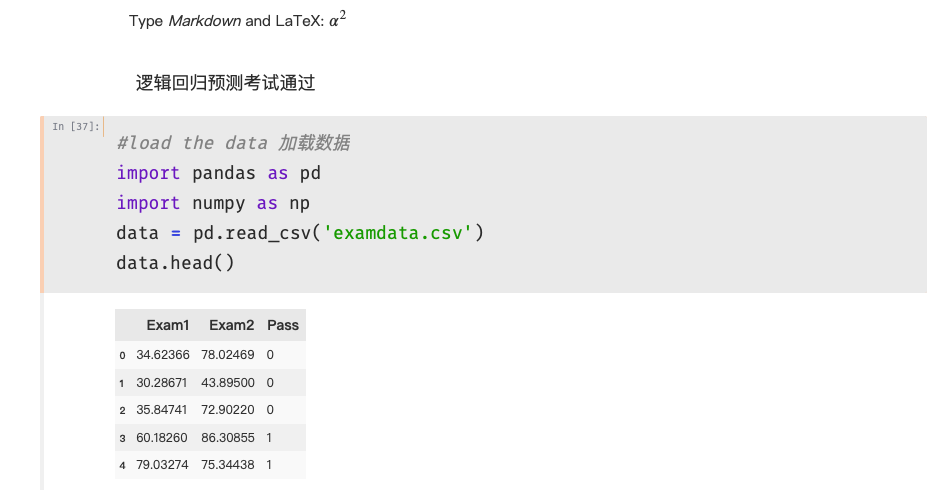
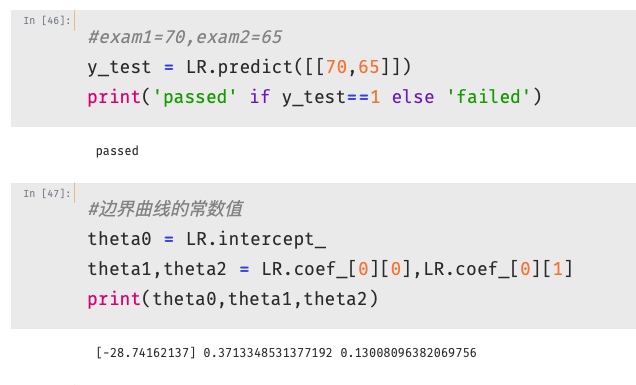
- 考试通过实战

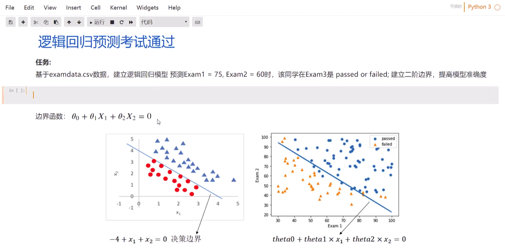
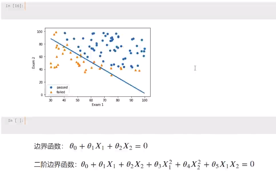
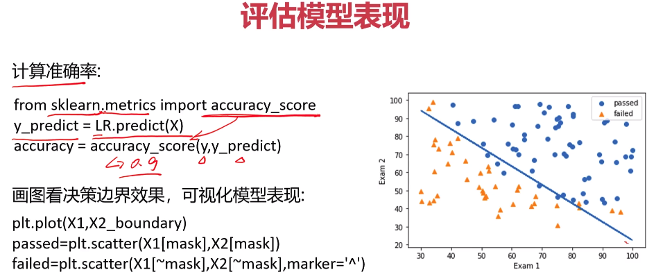
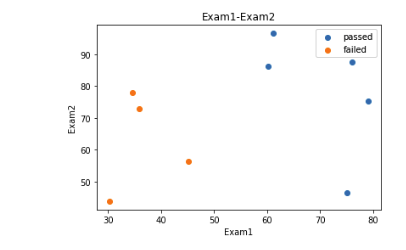
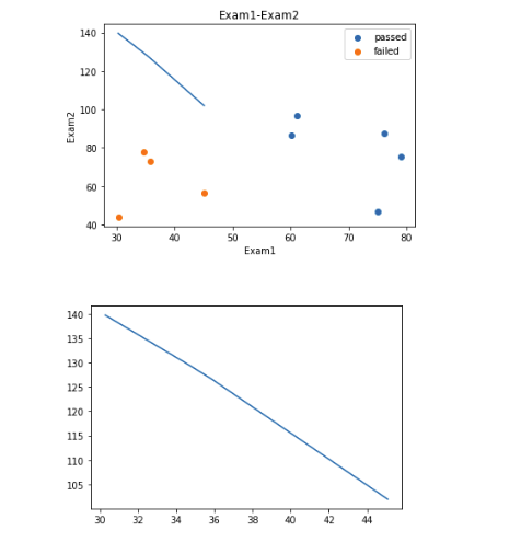
1 fig2 = plt.figure() #新建图形
2 passed = plt.scatter(data.loc[:,'Exam1'][mask],data.loc[:,'Exam2'][mask])#绘制散点图:展示通过考生的成绩
3 failed = plt.scatter(data.loc[:,'Exam1'][~mask],data.loc[:,'Exam2'][~mask])#绘制散点图:展示通过考生的成绩
4 plt.title('Exam1-Exam2')#标题
5 plt.xlabel('Exam1')#x轴
6 plt.ylabel('Exam2')#y轴
7 plt.legend((passed,failed),('passed','failed'))#题注
8 plt.show()#展示

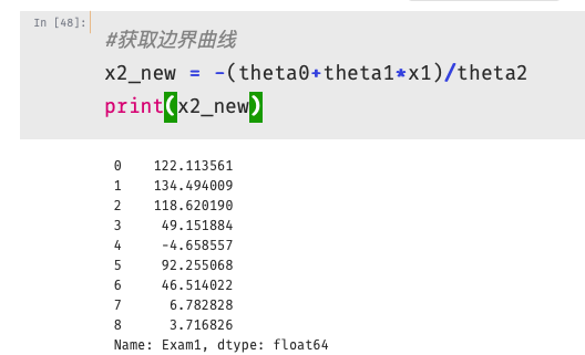
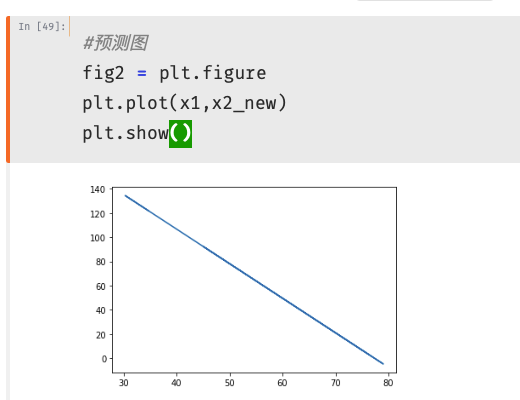
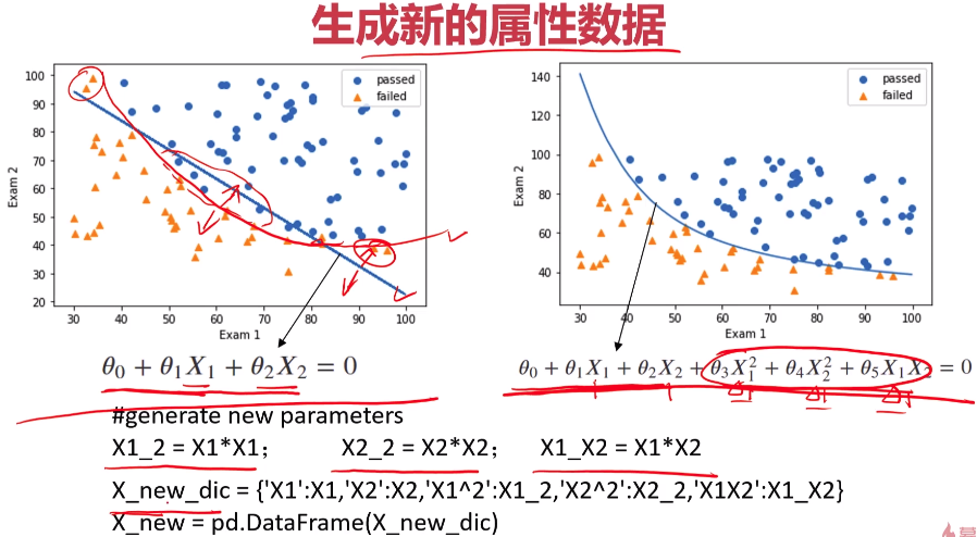
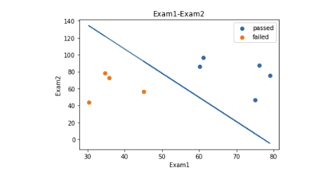
 1 #原始数据图
 2 fig3 = plt.figure() #新建图形
 3 passed = plt.scatter(data.loc[:,'Exam1'][mask],data.loc[:,'Exam2'][mask])#绘制散点图:展示通过考生的成绩
 4 failed = plt.scatter(data.loc[:,'Exam1'][~mask],data.loc[:,'Exam2'][~mask])#绘制散点图:展示通过考生的成绩
 5 plt.plot(x1,x2_new)#预测曲线
 6 plt.title('Exam1-Exam2')#标题
 7 plt.xlabel('Exam1')#x轴
 8 plt.ylabel('Exam2')#y轴
 9 plt.legend((passed,failed),('passed','failed'))#题注
10 plt.show()#展示
1 #绘制边界图形
2 theta0 = LR2.intercept_
3 theta1,theta2,theta3,theta4,theta5 = LR2.coef_[0][0],LR2.coef_[0][1],LR2.coef_[0][2],LR2.coef_[0][3],LR2.coef_[0][4]
4 a = theta4
5 b = theta5*x1_new+theta2
6 c = theta0+theta1*x1_new+theta3*x1_new*x1_new
7 x2_new_boundary = (-b+np.sqrt(b*b-4*a*c))/(2*a) # abs():取绝对值
8 print(x2_new_boundary)
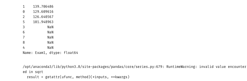
 1 #将原始数据与多阶函数进行混合
 2 fig5 = plt.figure() #新建图形
 3 passed = plt.scatter(data.loc[:,'Exam1'][mask],data.loc[:,'Exam2'][mask])#绘制散点图:展示通过考生的成绩
 4 failed = plt.scatter(data.loc[:,'Exam1'][~mask],data.loc[:,'Exam2'][~mask])#绘制散点图:展示通过考生的成绩
 5 plt.plot(x1_new,x2_new_boundary)#预测曲线
 6 plt.title('Exam1-Exam2')#标题
 7 plt.xlabel('Exam1')#x轴
 8 plt.ylabel('Exam2')#y轴
 9 plt.legend((passed,failed),('passed','failed'))#题注
10 plt.show()
11
12 plt.plot(x1_new,x2_new_boundary)
13 plt.show()
- 实战:芯片质量预测


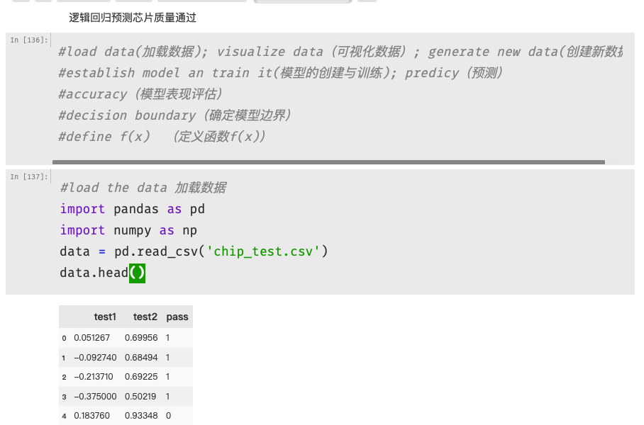
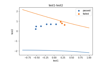
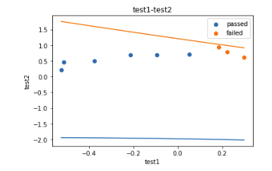
 1 #visualize the data 可视化数据 (数据展示可视化在Jupyter)
 2 %matplotlib inline
 3 from matplotlib import pyplot as plt
 4 fig1 = plt.figure() #新建图形
 5 passed = plt.scatter(data.loc[:,'test1'][mask],data.loc[:,'test2'][mask])#绘制散点图
 6 failed = plt.scatter(data.loc[:,'test1'][~mask],data.loc[:,'test2'][~mask])#绘制散点图
 7 plt.title('test1-test2')#标题
 8 plt.xlabel('test1')#x轴
 9 plt.ylabel('test2')#y轴
10 plt.legend((passed,failed),('passed','failed'))#题注
11 plt.show()#展示

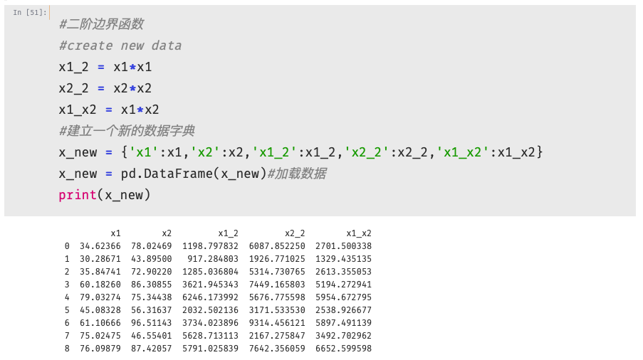
 1 #define x,y
 2 x = data.drop(['pass'],axis=1)#去除'pass'列
 3 y = data.loc[:,'pass']
 4 x1 = data.loc[:,'test1']
 5 x2 = data.loc[:,'test2']
 6 x1.head()
 7
 8 #二阶边界函数
 9 #create new data
10 x1_2 = x1*x1
11 x2_2 = x2*x2
12 x1_x2 = x1*x2
13 #建立一个新的数据字典
14 x_new = {'x1':x1,'x2':x2,'x1_2':x1_2,'x2_2':x2_2,'x1_x2':x1_x2}
15 x_new = pd.DataFrame(x_new)#加载数据
16 print(x_new)

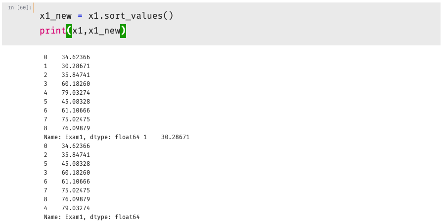
 1 x1_new = x1.sort_values()
 2 theta0 = LR2.intercept_
 3 theta1,theta2,theta3,theta4,theta5 = LR2.coef_[0][0],LR2.coef_[0][1],LR2.coef_[0][2],LR2.coef_[0][3],LR2.coef_[0][4]
 4 a = theta4
 5 b = theta5*x1_new+theta2
 6 c = theta0+theta1*x1_new+theta3*x1_new*x1_new
 7 x2_new_boundary = (-b+np.sqrt(b*b-4*a*c))/(2*a) # abs():取绝对值
 8
 9 #将原始数据与多阶函数进行混合
10 fig2 = plt.figure() #新建图形
11 passed = plt.scatter(data.loc[:,'test1'][mask],data.loc[:,'test2'][mask])#绘制散点图
12 failed = plt.scatter(data.loc[:,'test1'][~mask],data.loc[:,'test2'][~mask])#绘制散点图
13 plt.plot(x1_new,x2_new_boundary)#预测曲线
14 plt.title('test1-test2')#标题
15 plt.xlabel('test1')#x轴
16 plt.ylabel('test2')#y轴
17 plt.legend((passed,failed),('passed','failed'))#题注
18 plt.show()


 1 #将原始数据与多阶函数进行混合
 2 fig3 = plt.figure() #新建图形
 3 passed = plt.scatter(data.loc[:,'test1'][mask],data.loc[:,'test2'][mask])#绘制散点图
 4 failed = plt.scatter(data.loc[:,'test1'][~mask],data.loc[:,'test2'][~mask])#绘制散点图
 5 plt.plot(x1_new,x2_new_boundary1)#预测曲线
 6 plt.plot(x1_new,x2_new_boundary2)#预测曲线
 7 plt.title('test1-test2')#标题
 8 plt.xlabel('test1')#x轴
 9 plt.ylabel('test2')#y轴
10 plt.legend((passed,failed),('passed','failed'))#题注
11 plt.show()
1 x1_range = [-0.9 + x/10000 for x in range(0,19000)]
2 x1_range = np.array(x1_range)
3 x2_new_boundary1 = []
4 x2_new_boundary2 = []
5 for x in x1_range:
6     x2_new_boundary1.append(f(x)[0])
7     x2_new_boundary2.append(f(x)[1])
 1 #将原始数据与多阶函数进行混合
 2 fig4 = plt.figure() #新建图形
 3 passed = plt.scatter(data.loc[:,'test1'][mask],data.loc[:,'test2'][mask])#绘制散点图
 4 failed = plt.scatter(data.loc[:,'test1'][~mask],data.loc[:,'test2'][~mask])#绘制散点图
 5 plt.plot(x1_range,x2_new_boundary1)#预测曲线
 6 plt.plot(x1_range,x2_new_boundary2)#预测曲线
 7 plt.title('test1-test2')#标题
 8 plt.xlabel('test1')#x轴
 9 plt.ylabel('test2')#y轴
10 plt.legend((passed,failed),('passed','failed'))#题注
11 plt.show()