A* Search Algorithm

A* Search Algorithm

https://www.geeksforgeeks.org/a-search-algorithm/?ref=lbp

目标：

在存在障碍设置的空间中做路径搜索。

除了这个算法，还有其它搜索算法，见

https://www.cs.cmu.edu/~motionplanning/lecture/AppH-astar-dstar_howie.pdf

Motivation 
To approximate the shortest path in real-life situations, like- in maps, games where there can be many hindrances.
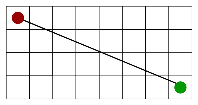
We can consider a 2D Grid having several obstacles and we start from a source cell (colored red below) to reach towards a goal cell (colored green below)

A* 不同于其它遍历算法的地方是， 这个方法拥有大脑， 可以快速的搜索出近似最短路。

What is A* Search Algorithm? 
A* Search algorithm is one of the best and popular technique used in path-finding and graph traversals.

 

Why A* Search Algorithm? 
Informally speaking, A* Search algorithms, unlike other traversal techniques, it has “brains”. What it means is that it is really a smart algorithm which separates it from the other conventional algorithms. This fact is cleared in detail in below sections. 
And it is also worth mentioning that many games and web-based maps use this algorithm to find the shortest path very efficiently (approximation).

评判函数f由两部分组成g和h

g是从开始节点到当前节点的最小花费。

h是从当前节点到目标节点的估算花费。

Explanation 
Consider a square grid having many obstacles and we are given a starting cell and a target cell. We want to reach the target cell (if possible) from the starting cell as quickly as possible. Here A* Search Algorithm comes to the rescue.
What A* Search Algorithm does is that at each step it picks the node according to a value-‘f’ which is a parameter equal to the sum of two other parameters – ‘g’ and ‘h’. At each step it picks the node/cell having the lowest ‘f’, and process that node/cell.
We define ‘g’ and ‘h’ as simply as possible below
g = the movement cost to move from the starting point to a given square on the grid, following the path generated to get there. 
h = the estimated movement cost to move from that given square on the grid to the final destination. This is often referred to as the heuristic, which is nothing but a kind of smart guess. We really don’t know the actual distance until we find the path, because all sorts of things can be in the way (walls, water, etc.). There can be many ways to calculate this ‘h’ which are discussed in the later sections.

详细的过程

主要对象为两个 openlist 和 closelist

openlist为启发式搜索找到的可能距离目标状态的中间节点

closelist为从openlist中选拔出来的最小路径节点

选拔过程采用优先队列。

Algorithm 
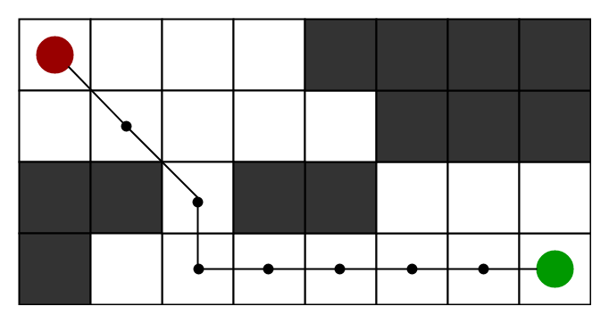
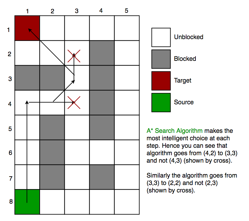
We create two lists – Open List and Closed List (just like Dijkstra Algorithm)  

// A* Search Algorithm
1.  Initialize the open list
2.  Initialize the closed list
    put the starting node on the open 
    list (you can leave its f at zero)

3.  while the open list is not empty
    a) find the node with the least f on 
       the open list, call it "q"

    b) pop q off the open list
  
    c) generate q's 8 successors and set their 
       parents to q
   
    d) for each successor
        i) if successor is the goal, stop search
        
        ii) else, compute both g and h for successor
          successor.g = q.g + distance between 
                              successor and q
          successor.h = distance from goal to 
          successor (This can be done using many 
          ways, we will discuss three heuristics- 
          Manhattan, Diagonal and Euclidean 
          Heuristics)
          
          successor.f = successor.g + successor.h

        iii) if a node with the same position as 
            successor is in the OPEN list which has a 
           lower f than successor, skip this successor

        iV) if a node with the same position as 
            successor  is in the CLOSED list which has
            a lower f than successor, skip this successor
            otherwise, add  the node to the open list
     end (for loop)
  
    e) push q on the closed list
    end (while loop)

So suppose as in the below figure if we want to reach the target cell from the source cell, then the A* Search algorithm would follow path as shown below. Note that the below figure is made by considering Euclidean Distance as a heuristics.

启发式分类两种：

一种为确定启发式，这个我认为不能算是启发式了，因为当前节点到目标节点的最小距离计算出来了

另一种为近似启发式， 采用距离度量： 欧几里得距离 曼哈顿距离 。。。

Heuristics 
We can calculate g but how to calculate h ?
We can do things. 
A) Either calculate the exact value of h (which is certainly time consuming). 
             OR 
B ) Approximate the value of h using some heuristics (less time consuming).
We will discuss both of the methods.
A) Exact Heuristics –
We can find exact values of h, but that is generally very time consuming.
Below are some of the methods to calculate the exact value of h.
1) Pre-compute the distance between each pair of cells before running the A* Search Algorithm.
2) If there are no blocked cells/obstacles then we can just find the exact value of h without any pre-computation using the distance formula/Euclidean Distance

B) Approximation Heuristics – 
There are generally three approximation heuristics to calculate h –

1) Manhattan Distance –  

• It is nothing but the sum of absolute values of differences in the goal’s x and y coordinates and the current cell’s x and y coordinates respectively, i.e.,

 h = abs (current_cell.x – goal.x) + 
     abs (current_cell.y – goal.y)

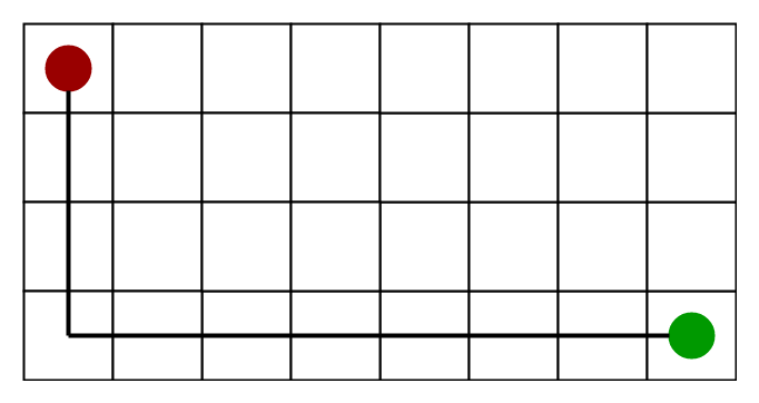
• When to use this heuristic? – When we are allowed to move only in four directions only (right, left, top, bottom)

The Manhattan Distance Heuristics is shown by the below figure (assume red spot as source cell and green spot as target cell). 

2) Diagonal Distance- 

• It is nothing but the maximum of absolute values of differences in the goal’s x and y coordinates and the current cell’s x and y coordinates respectively, i.e.,

dx = abs(current_cell.x – goal.x)
dy = abs(current_cell.y – goal.y)
 
h = D * (dx + dy) + (D2 - 2 * D) * min(dx, dy)

where D is length of each node(usually = 1) and D2 is diagonal distance between each node (usually = sqrt(2) ). 

• When to use this heuristic? – When we are allowed to move in eight directions only (similar to a move of a King in Chess)

The Diagonal Distance Heuristics is shown by the below figure (assume red spot as source cell and green spot as target cell).
 

3) Euclidean Distance-

• As it is clear from its name, it is nothing but the distance between the current cell and the goal cell using the distance formula

 h = sqrt ( (current_cell.x – goal.x)2 + 
            (current_cell.y – goal.y)2 )

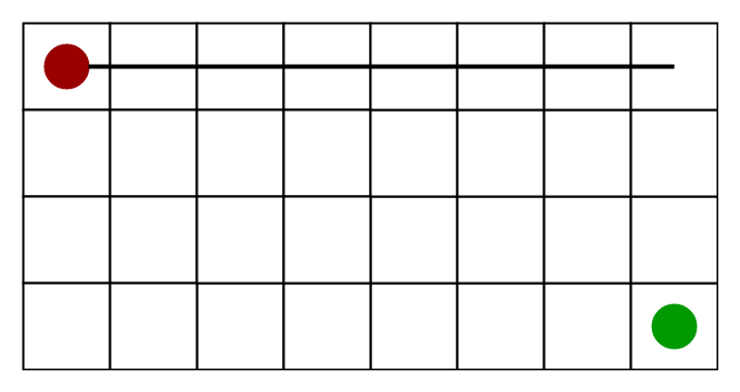
• When to use this heuristic? – When we are allowed to move in any directions.

The Euclidean Distance Heuristics is shown by the below figure (assume red spot as source cell and green spot as target cell).

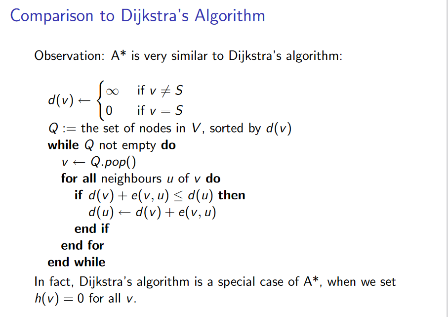
Relation (Similarity and Differences) with other algorithms- 
Dijkstra is a special case of A* Search Algorithm, where h = 0 for all nodes.

此方法搜索出来的路径，可能为最短路径，也可能不是。

Limitations 
Although being the best path finding algorithm around, A* Search Algorithm doesn’t produce the shortest path always, as it relies heavily on heuristics / approximations to calculate – h

Applications 
This is the most interesting part of A* Search Algorithm. They are used in games! But how?
Ever played Tower Defense Games ? 
Tower defense is a type of strategy video game where the goal is to defend a player’s territories or possessions by obstructing enemy attackers, usually achieved by placing defensive structures on or along their path of attack. 
A* Search Algorithm is often used to find the shortest path from one point to another point. You can use this for each enemy to find a path to the goal.
One example of this is the very popular game- Warcraft III

时间复杂度，最坏可能所有边都有遍历到

空间复杂度，最坏情况所有的点都要入队列

Time Complexity 
Considering a graph, it may take us to travel all the edge to reach the destination cell from the source cell [For example, consider a graph where source and destination nodes are connected by a series of edges, like – 0(source) –>1 –> 2 –> 3 (target)
So the worse case time complexity is O(E), where E is the number of edges in the graph

Auxiliary Space In the worse case we can have all the edges inside the open list, so required auxiliary space in worst case is O(V), where V is the total number of vertices.

单个开始节点-单个目标节点， 用此方法

单个开始节点-所有的目标节点，用BFS DIJKSTRA Bellman

任何节点之间，用 Floyd-warshall

Summary 
So when to use BFS over A*, when to use Dijkstra over A* to find the shortest paths ? 
We can summarise this as below-
1) One source and One Destination- 
→ Use A* Search Algorithm (For Unweighted as well as Weighted Graphs)
2) One Source, All Destination – 
→ Use BFS (For Unweighted Graphs) 
→ Use Dijkstra (For Weighted Graphs without negative weights) 
→ Use Bellman Ford (For Weighted Graphs with negative weights)
3) Between every pair of nodes- 
→ Floyd-Warshall 
→ Johnson’s Algorithm

Dijkstra是A星的一种特殊情况

https://courses.cs.duke.edu/fall11/cps149s/notes/a_star.pdf

8-puzzle problem

https://www.gatevidyalay.com/tag/a-star-search-algorithm-example/

Given an initial state of a 8-puzzle problem and final state to be reached-

Find the most cost-effective path to reach the final state from initial state using A* Algorithm.

Consider g(n) = Depth of node and h(n) = Number of misplaced tiles.

Solution-

• A* Algorithm maintains a tree of paths originating at the initial state.
• It extends those paths one edge at a time.
• It continues until final state is reached.

 

Introduction to the A* Algorithm

https://www.redblobgames.com/pathfinding/a-star/introduction.html

交互式的方式演示扩展过程。非常推荐初学者理解。

There are lots of algorithms that run on graphs. I’m going to cover these:

	Breadth First Search explores equally in all directions. This is an incredibly useful algorithm, not only for regular path finding, but also for procedural map generation, flow field pathfinding, distance maps, and other types of map analysis.
	Dijkstra’s Algorithm (also called Uniform Cost Search) lets us prioritize which paths to explore. Instead of exploring all possible paths equally, it favors lower cost paths. We can assign lower costs to encourage moving on roads, higher costs to avoid forests, higher costs to discourage going near enemies, and more. When movement costs vary, we use this instead of Breadth First Search.
	A* is a modification of Dijkstra’s Algorithm that is optimized for a single destination. Dijkstra’s Algorithm can find paths to all locations; A* finds paths to one location, or the closest of several locations. It prioritizes paths that seem to be leading closer to a goal.

I’ll start with the simplest, Breadth First Search, and add one feature at a time to turn it into A*.

Which algorithm should you use for finding paths on a game map?

• If you want to find paths from or to all all locations, use Breadth First Search or Dijkstra’s Algorithm. Use Breadth First Search if movement costs are all the same; use Dijkstra’s Algorithm if movement costs vary.
• If you want to find paths to one location, or the closest of several goals, use Greedy Best First Search or A*. Prefer A* in most cases. When you’re tempted to use Greedy Best First Search, consider using A* with an “inadmissible” heuristic.

What about optimal paths? Breadth First Search and Dijkstra’s Algorithm are guaranteed to find the shortest path given the input graph. Greedy Best First Search is not. A* is guaranteed to find the shortest path if the heuristic is never larger than the true distance. As the heuristic becomes smaller, A* turns into Dijkstra’s Algorithm. As the heuristic becomes larger, A* turns into Greedy Best First Search.

What about performance? The best thing to do is to eliminate unnecessary locations in your graph. If using a grid, see this. Reducing the size of the graph helps all the graph search algorithms. After that, use the simplest algorithm you can; simpler queues run faster. Greedy Best First Search typically runs faster than Dijkstra’s Algorithm but doesn’t produce optimal paths. A* is a good choice for most pathfinding needs.

算法适用性分类

https://www.redblobgames.com/pathfinding/tower-defense/

Graph search algorithms like A* are often used to find the shortest path from one point to another point. You can use this for each enemy to find a path to the goal. There are lots of different graph search algorithms we could use in this type of game. These are the classics:

1. One source, one destination:
   • Greedy Best First Search
   • A* - commonly used in games
2. One source, all destinations, or all sources, one destination:
   • Breadth First Search - unweighted edges
   • Dijkstra’s Algorithm - adds weights to edges
   • Bellman-Ford - supports negative weights
3. All sources, all destinations:
   • Floyd-Warshall
   • Johnson’s Algorithm