MINST手写数字识别（一）—— 全连接网络

这是一个简单快速入门教程——用Keras搭建神经网络实现手写数字识别，它大部分基于Keras的源代码示例 minst_mlp.py.

1、安装依赖库

首先，你需要安装最近版本的Python，再加上一些包Keras,numpy,matplotlib和jupyter.你可以安装这些报在全局，但是我建议安装它们在virtualenv虚拟环境，

这基本上封装了一个完全孤立的Python环境。

安装Python包管理器

sudo easy_install pip

安装virtualenv

pip install virtualenv

使用cd ~进入主目录，并创建一个名为kerasenv的虚拟环境

virtualenv kerasenv

再激活这个虚拟环境

source kerasenv/bin/activate

现在你可以安装前面提到的包到这个环境

pip install numpy jupyter keras matplotlib

2、搭建神经网络

以下代码都在Google Colab中运行

2.1 导入一些依赖

import numpy as np
import matplotlib.pyplot as plt
plt.rcParams['figure.figsize'] = (7,7) # Make the figures a bit bigger

from keras.datasets import mnist
from keras.models import Sequential
from keras.layers.core import Dense, Dropout, Activation
from keras.utils import np_utils

 2.2 装载训练数据

nb_classes = 10

# the data, shuffled and split between tran and test sets
(X_train, y_train), (X_test, y_test) = mnist.load_data()
print("X_train original shape", X_train.shape)
print("y_train original shape", y_train.shape)

结果：

Downloading data from https://s3.amazonaws.com/img-datasets/mnist.npz
11493376/11490434 [==============================] - 0s 0us/step
X_train original shape (60000, 28, 28)
y_train original shape (60000,)

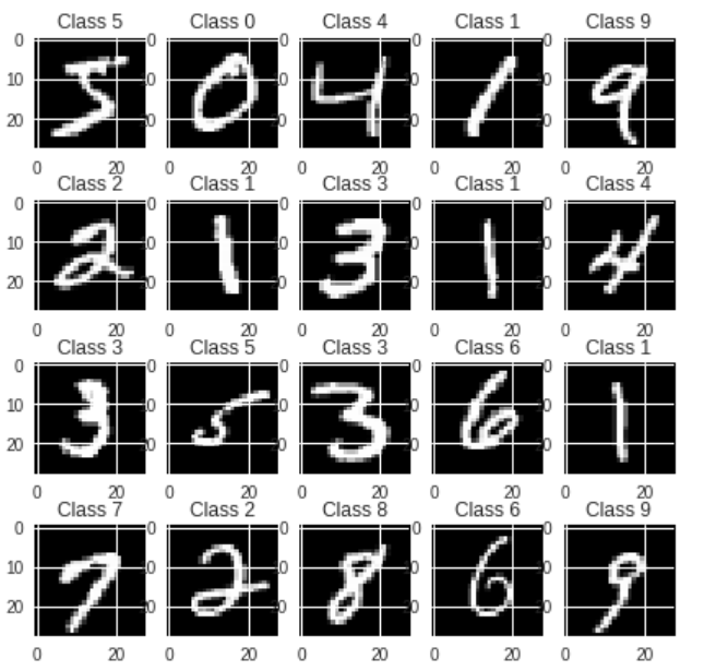
让我们看看训练集中的一些例子：

for i in range(20):
    plt.subplot(4,5,i+1)
    plt.imshow(X_train[i], cmap='gray', interpolation='none')
    plt.title("Class {}".format(y_train[i]))

 2.3 格式化训练数据

对于每一个训练样本我们的神经网络得到单个的数组，所以我们需要将28x28的图片变形成784的向量，我们还将输入从[0,255]缩到[0,1].

X_train = X_train.reshape(60000, 784)
X_test = X_test.reshape(10000, 784)
X_train = X_train.astype('float32')
X_test = X_test.astype('float32')
X_train /= 255
X_test /= 255
print("Training matrix shape", X_train.shape)
print("Testing matrix shape", X_test.shape)

结果：

Training matrix shape (60000, 784)
Testing matrix shape (10000, 784)

将目标矩阵变成one-hot格式

0 -> [1, 0, 0, 0, 0, 0, 0, 0, 0]
1 -> [0, 1, 0, 0, 0, 0, 0, 0, 0]
2 -> [0, 0, 1, 0, 0, 0, 0, 0, 0]
etc.

Y_train = np_utils.to_categorical(y_train, nb_classes)
Y_test = np_utils.to_categorical(y_test, nb_classes)

2.4 搭建神经网络

2.4.1  搭建三层全连接网络

我们将做一个简单的三层全连接网络，如下：

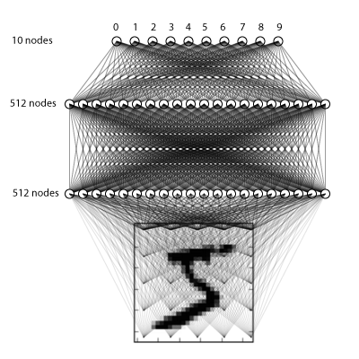
model = Sequential()
model.add(Dense(512, input_shape=(784,)))
model.add(Activation('relu')) # An "activation" is just a non-linear function applied to the output
                              # of the layer above. Here, with a "rectified linear unit",
                              # we clamp all values below 0 to 0.
                           
model.add(Dropout(0.2))   # Dropout helps protect the model from memorizing or "overfitting" the training data
model.add(Dense(512))
model.add(Activation('relu'))
model.add(Dropout(0.2))
model.add(Dense(10))
model.add(Activation('softmax')) # This special "softmax" activation among other things,
                                 # ensures the output is a valid probaility distribution, that is
                                 # that its values are all non-negative and sum to 1.

结果：

WARNING:tensorflow:From /usr/local/lib/python3.6/dist-packages/tensorflow/python/framework/op_def_library.py:263: colocate_with (from tensorflow.python.framework.ops) is deprecated and will be removed in a future version.
Instructions for updating:
Colocations handled automatically by placer.
WARNING:tensorflow:From /usr/local/lib/python3.6/dist-packages/keras/backend/tensorflow_backend.py:3445: calling dropout (from tensorflow.python.ops.nn_ops) with keep_prob is deprecated and will be removed in a future version.
Instructions for updating:
Please use `rate` instead of `keep_prob`. Rate should be set to `rate = 1 - keep_prob`.

2.4.2  编译模型

      Keras是建立在Theano（现在TensorFlow也是），这两个包都允许你定义计算图，然后高效地在CPU或GPU上编译和运行，而没有Python解释器地开销。

      当编译一个模型，Keras要求你确定损失函数和优化器，我使用的是分类交叉熵（categorical crossentropy），它是一种非常适合比较两个概率分布的函数。

      在这里，我们的预测是十个不同数字的概率分布（例如，80%认为这个图片是3，10%认为是2，5%认为是1等），目标是一个概率分布，正确类别为100％，其他所有类别为0。交叉熵是度量两个概率分布差异程度的方法，详情wiki。

      优化器帮助模型快速的学习，同时防止“卡住“和“爆炸”的情况，我们不讨论其太多的细节，但是“adam”是一个经常使用的好的选择。

model.compile(loss='categorical_crossentropy', optimizer='adam')

2.4.3  训练模型！

这是有趣的部分：你可以喂入之前加载好的训练集到模型，它将学习如何分类数字.

model.fit(X_train, Y_train,
          batch_size=128, epochs=4,
          verbose=1,
          validation_data=(X_test, Y_test))

结果：

Train on 60000 samples, validate on 10000 samples
Epoch 1/4
60000/60000 [==============================] - 10s 171us/step - loss: 0.0514 - val_loss: 0.0691
Epoch 2/4
60000/60000 [==============================] - 10s 170us/step - loss: 0.0410 - val_loss: 0.0700
Epoch 3/4
60000/60000 [==============================] - 11s 177us/step - loss: 0.0349 - val_loss: 0.0750
Epoch 4/4
60000/60000 [==============================] - 11s 184us/step - loss: 0.0298 - val_loss: 0.0616
<keras.callbacks.History at 0x7f531f596fd0>

2.4.4  最后，评估其性能

score = model.evaluate(X_test, Y_test,
                       verbose=0)
print('Test score:', score)

效果：

Test score: 0.061617326979574866

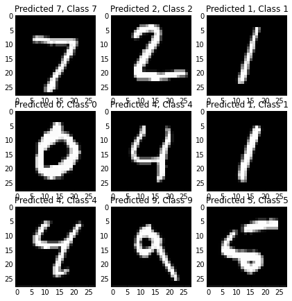
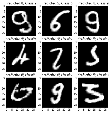
检查输出，检查输出并确保一切看起来都很合理，这总是一个好主意。接下来，我们看一些分类正确的例子和错误的例子.

# The predict_classes function outputs the highest probability class
# according to the trained classifier for each input example.
predicted_classes = model.predict_classes(X_test)

# Check which items we got right / wrong
correct_indices = np.nonzero(predicted_classes == y_test)[0]
incorrect_indices = np.nonzero(predicted_classes != y_test)[0]

plt.figure()
for i, correct in enumerate(correct_indices[:9]):
    plt.subplot(3,3,i+1)
    plt.imshow(X_test[correct].reshape(28,28), cmap='gray', interpolation='none')
    plt.title("Predicted {}, Class {}".format(predicted_classes[correct], y_test[correct]))
    
plt.figure()
for i, incorrect in enumerate(incorrect_indices[:9]):
    plt.subplot(3,3,i+1)
    plt.imshow(X_test[incorrect].reshape(28,28), cmap='gray', interpolation='none')
    plt.title("Predicted {}, Class {}".format(predicted_classes[incorrect], y_test[incorrect]))

结果：

总之，这是一个完整的程序，在Keras主页http://keras.io/和githubhttps://github.com/fchollet/keras有其它许多优秀的例子。