《DSP using MATLAB》Problem 9.2

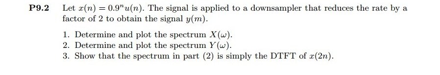
        前几天看了看博客，从16年底到现在，3年了，终于看书到第9章了。都怪自己愚钝不堪，唯有吃苦努力，一点一点一页一页慢慢啃了。

代码：

%% ------------------------------------------------------------------------
%%            Output Info about this m-file
fprintf('
***********************************************************
');
fprintf('        <DSP using MATLAB> Problem 9.2 

');

banner();
%% ------------------------------------------------------------------------


% ------------------------------------------------------------
%                  PART 1   
% ------------------------------------------------------------

% Discrete time signal

n1_start = 0; n1_end = 60;
      n1 = [n1_start:1:n1_end];
    
xn1 = (0.9).^n1 .* stepseq(0, n1_start, n1_end);             % digital signal

 D = 2;                      % downsample by factor D 
 y = downsample(xn1, D);
ny = [n1_start:n1_end/D];

figure('NumberTitle', 'off', 'Name', 'Problem 9.2 xn1 and y')
set(gcf,'Color','white'); 
subplot(2,1,1); stem(n1, xn1, 'b');
xlabel('n'); ylabel('x(n)');
title('xn1 original sequence');  grid on;
subplot(2,1,2); stem(ny, y, 'r');
xlabel('ny'); ylabel('y(n)');
title('y sequence, downsample by D=2 ');  grid on;


% ----------------------------
%       DTFT of xn1
% ----------------------------
M = 500;
[X1, w] = dtft1(xn1, n1, M);

magX1  = abs(X1);  angX1  = angle(X1);  realX1  = real(X1);  imagX1  = imag(X1);


%% --------------------------------------------------------------------
%%              START X(w)'s  mag ang real imag
%% --------------------------------------------------------------------
figure('NumberTitle', 'off', 'Name', 'Problem 9.2 X1 DTFT');
set(gcf,'Color','white'); 
subplot(2,1,1); plot(w/pi,magX1); grid on;  %axis([-1,1,0,1.05]); 
title('Magnitude Response');
xlabel('digital frequency in pi units'); ylabel('Magnitude  |H|'); 
subplot(2,1,2); plot(w/pi, angX1/pi); grid on;  %axis([-1,1,-1.05,1.05]);
title('Phase Response');
xlabel('digital frequency in pi units'); ylabel('Radians/pi');

figure('NumberTitle', 'off', 'Name', 'Problem 9.2 X1 DTFT');
set(gcf,'Color','white'); 
subplot(2,1,1); plot(w/pi, realX1); grid on;
title('Real Part');
xlabel('digital frequency in pi units'); ylabel('Real');
subplot(2,1,2); plot(w/pi, imagX1); grid on;
title('Imaginary Part');
xlabel('digital frequency in pi units'); ylabel('Imaginary');
%% -------------------------------------------------------------------
%%             END X's  mag ang real imag
%% -------------------------------------------------------------------


% ----------------------------
%       DTFT of y
% ----------------------------
M = 500;
[Y, w] = dtft1(y, ny, M);

magY_DTFT = abs(Y);  angY_DTFT = angle(Y);  realY_DTFT = real(Y);  imagY_DTFT = imag(Y);


%% --------------------------------------------------------------------
%%              START Y(w)'s  mag ang real imag
%% --------------------------------------------------------------------
figure('NumberTitle', 'off', 'Name', 'Problem 9.2 Y DTFT');
set(gcf,'Color','white'); 
subplot(2,1,1); plot(w/pi, magY_DTFT); grid on;  %axis([-1,1,0,1.05]); 
title('Magnitude Response');
xlabel('digital frequency in pi units'); ylabel('Magnitude  |H|'); 
subplot(2,1,2); plot(w/pi, angY_DTFT/pi); grid on;  %axis([-1,1,-1.05,1.05]);
title('Phase Response');
xlabel('digital frequency in pi units'); ylabel('Radians/pi');

figure('NumberTitle', 'off', 'Name', 'Problem 9.2 Y DTFT');
set(gcf,'Color','white'); 
subplot(2,1,1); plot(w/pi, realY_DTFT); grid on;
title('Real Part');
xlabel('digital frequency in pi units'); ylabel('Real');
subplot(2,1,2); plot(w/pi, imagY_DTFT); grid on;
title('Imaginary Part');
xlabel('digital frequency in pi units'); ylabel('Imaginary');
%% -------------------------------------------------------------------
%%             END Y's  mag ang real imag
%% -------------------------------------------------------------------



figure('NumberTitle', 'off', 'Name', 'Problem 9.2 X1 & Y, DTFT of x and y');
set(gcf,'Color','white'); 
subplot(2,1,1); plot(w/pi,magX1); grid on;  %axis([-1,1,0,1.05]); 
title('Magnitude Response');
xlabel('digital frequency in pi units'); ylabel('Magnitude  |H|');  
hold on;
plot(w/pi, magY_DTFT, 'r'); gtext('magY(omega)', 'Color', 'r');
hold off;

subplot(2,1,2); plot(w/pi, angX1/pi); grid on;  %axis([-1,1,-1.05,1.05]);
title('Phase Response');
xlabel('digital frequency in pi units'); ylabel('Radians/pi');
hold on;
plot(w/pi, angY_DTFT/pi, 'r'); gtext('AngY(omega)', 'Color', 'r');
hold off;

　　运行结果：

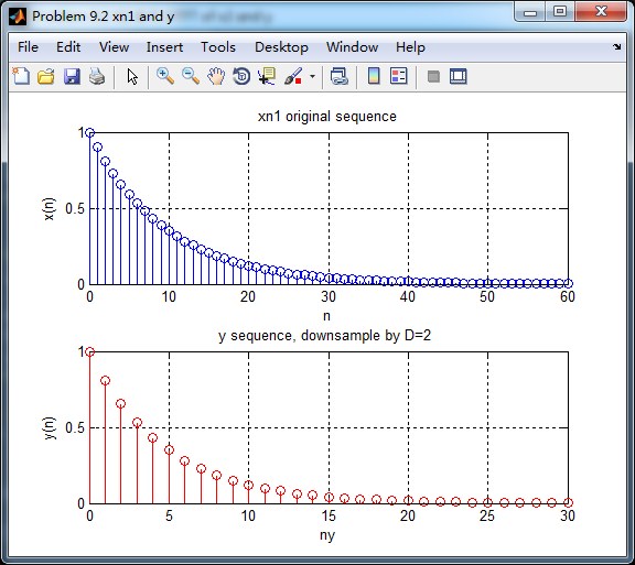
        原始序列x和按D=2抽取后序列y，如下

        原始序列x的DTFT，这里只放幅度谱和相位谱，DTFT的实部和虚部的图不放了（代码中有计算）。

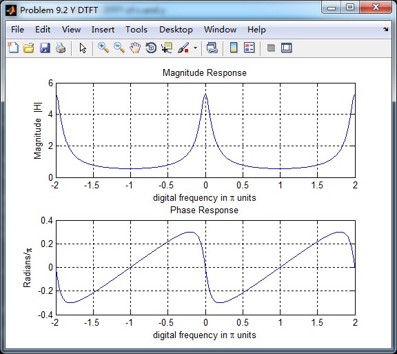
        抽取后序列y的DTFT如下图，也是幅度谱和相位谱，实部和虚部的图不放了（代码中有计算）。

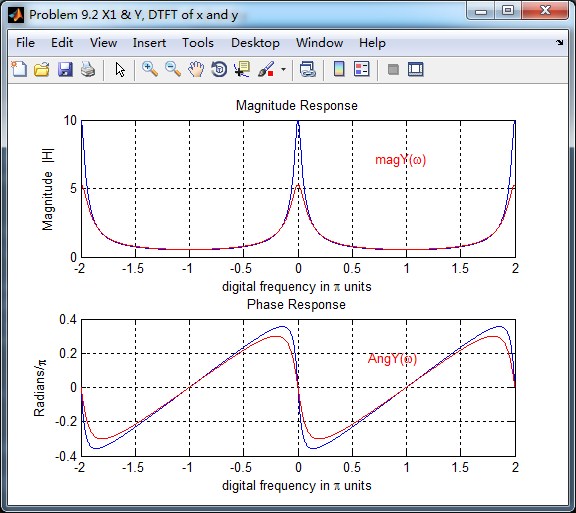
        将上述两张图叠合到一起做对比，红色曲线是抽取后序列的DTFT，蓝色曲线是原始序列的DTFT。

可见，红色曲线的幅度近似为蓝色曲线的二分之一（1/D，这里D=2）。