《DSP using MATLAB》Problem 7.14

代码：

%% ++++++++++++++++++++++++++++++++++++++++++++++++++++++++++++++++++++++++++++++++
%%            Output Info about this m-file
fprintf('
***********************************************************
');
fprintf('        <DSP using MATLAB> Problem 7.14 

');

banner();
%% ++++++++++++++++++++++++++++++++++++++++++++++++++++++++++++++++++++++++++++++++

% bandpass
ws1 = 0.25*pi; wp1 = 0.35*pi; wp2=0.65*pi; ws2=0.75*pi; 
delta1 = 0.05; delta2 = 0.01;
tr_width = min(wp1-ws1, ws2-wp2);
f = [ws1, wp1, wp2, ws2]/pi;

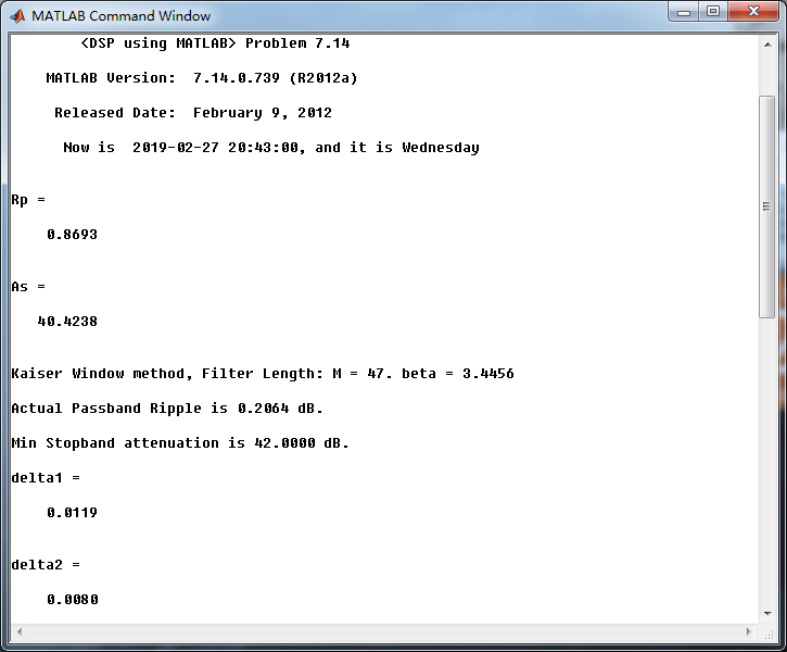
[Rp, As] = delta2db(delta1, delta2)

M = ceil((As-7.95)/(2.285*tr_width)) + 1;                 % Kaiser Window
if As > 21 || As < 50 
	beta = 0.5842*(As-21)^0.4 + 0.07886*(As-21);
else
	beta = 0.1102*(As-8.7);
end


fprintf('
Kaiser Window method, Filter Length: M = %d. beta = %.4f
', M, beta);


n = [0:1:M-1]; wc1 = (ws1+wp1)/2; wc2 = (ws2+wp2)/2;

%wc = (ws + wp)/2,                    % ideal LPF cutoff frequency

hd = ideal_lp(wc2, M) - ideal_lp(wc1, M); 
w_kai = (kaiser(M, beta))';  h = hd .* w_kai;
[db, mag, pha, grd, w] = freqz_m(h, [1]);  delta_w = 2*pi/1000;
[Hr,ww,P,L] = ampl_res(h);

Rp = -(min(db(wp1/delta_w :1: wp2/delta_w+1)));                            % Actual Passband Ripple
fprintf('
Actual Passband Ripple is %.4f dB.
', Rp);

As = -round(max(db(1 : 1 : floor(ws1/delta_w)+1 )));   % Min Stopband attenuation
fprintf('
Min Stopband attenuation is %.4f dB.
', As);

[delta1, delta2] = db2delta(Rp, As)


% Plot

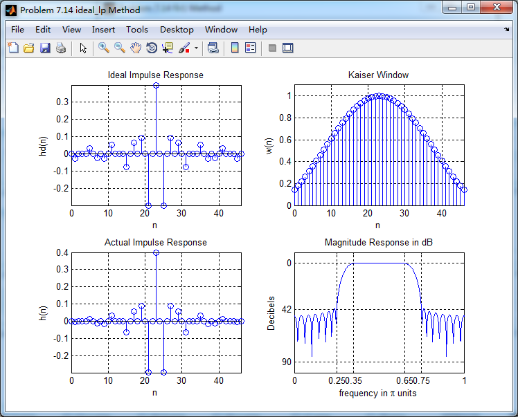
figure('NumberTitle', 'off', 'Name', 'Problem 7.14 ideal_lp Method')
set(gcf,'Color','white'); 

subplot(2,2,1); stem(n, hd); axis([0 M-1 -0.3 0.4]); grid on;
xlabel('n'); ylabel('hd(n)'); title('Ideal Impulse Response');

subplot(2,2,2); stem(n, w_kai); axis([0 M-1 0 1.1]); grid on;
xlabel('n'); ylabel('w(n)'); title('Kaiser Window');

subplot(2,2,3); stem(n, h); axis([0 M-1 -0.3 0.4]); grid on;
xlabel('n'); ylabel('h(n)'); title('Actual Impulse Response');

subplot(2,2,4); plot(w/pi, db); axis([0 1 -100 10]); grid on;
set(gca,'YTickMode','manual','YTick',[-90,-42,0]);
set(gca,'YTickLabelMode','manual','YTickLabel',['90';'42';' 0']);
set(gca,'XTickMode','manual','XTick',[0,f,1]);
xlabel('frequency in pi units'); ylabel('Decibels'); title('Magnitude Response in dB');


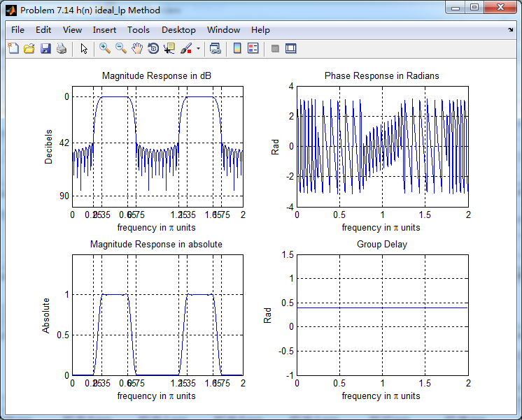
figure('NumberTitle', 'off', 'Name', 'Problem 7.14 h(n) ideal_lp Method')
set(gcf,'Color','white'); 

subplot(2,2,1); plot(w/pi, db); grid on; axis([0 2 -100 10]); 
xlabel('frequency in pi units'); ylabel('Decibels'); title('Magnitude Response in dB');
set(gca,'YTickMode','manual','YTick',[-90,-42,0])
set(gca,'YTickLabelMode','manual','YTickLabel',['90';'42';' 0']);
set(gca,'XTickMode','manual','XTick',[0,f,1+f,2]);

subplot(2,2,3); plot(w/pi, mag); grid on; %axis([0 2 -100 10]); 
xlabel('frequency in pi units'); ylabel('Absolute'); title('Magnitude Response in absolute');
set(gca,'XTickMode','manual','XTick',[0,f,1+f,2]);
set(gca,'YTickMode','manual','YTick',[0,0.5, 1])

subplot(2,2,2); plot(w/pi, pha); grid on; %axis([0 1 -100 10]); 
xlabel('frequency in pi units'); ylabel('Rad'); title('Phase Response in Radians');
subplot(2,2,4); plot(w/pi, grd*pi/180);  grid on; %axis([0 1 -100 10]); 
xlabel('frequency in pi units'); ylabel('Rad'); title('Group Delay');

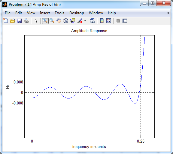
figure('NumberTitle', 'off', 'Name', 'Problem 7.14 Amp Res of h(n)')
set(gcf,'Color','white'); 

plot(ww/pi, Hr); grid on; %axis([0 1 -100 10]); 
xlabel('frequency in pi units'); ylabel('Hr'); title('Amplitude Response');
set(gca,'YTickMode','manual','YTick',[-delta2,0,delta2,1 - delta1,1, 1 + delta1])
%set(gca,'YTickLabelMode','manual','YTickLabel',['90';'45';' 0']);
set(gca,'XTickMode','manual','XTick',[0,f,2]);


%% +++++++++++++++++++++++++++++++++++++++++
%%          fir1 function method
%% +++++++++++++++++++++++++++++++++++++++++
f = [ws1, wp1, wp2, ws2]/pi;
m = [0 1 0];
ripple = [0.01 0.05 0.01];
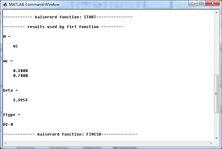
[N, wc, beta, ftype] = kaiserord(f,m,ripple);
fprintf('
------------ kaiserord function: START---------------
');
fprintf('
--------- results used by fir1 function ---------
');
N
wc
beta
ftype
fprintf('------------- kaiserord function: FINISH---------------
');
%h_check = fir1(M-1, [wc1 wc2]/pi, 'stop', window(@kaiser, M));
%h_check = fir1(N, wc, ftype, window(@kaiser, N+1));
h_check = fir1(N, wc, ftype, kaiser(N+1, beta));

[db, mag, pha, grd, w] = freqz_m(h_check, [1]);  
[Hr,ww,P,L] = ampl_res(h_check);

As = -round(max(db(1 : 1 : floor(ws1/delta_w)+1 )));   % Min Stopband attenuation
fprintf('
Min Stopband attenuation is %.4f dB.
', As);

Rp = -(min(db(wp1/delta_w :1: wp2/delta_w+1)));         % Actual Passband Ripple
fprintf('
Actual Passband Ripple is %.4f dB.
', Rp);

[delta1, delta2] = db2delta(Rp, As)

%% -------------------------------------------
%%     plot
%% -------------------------------------------
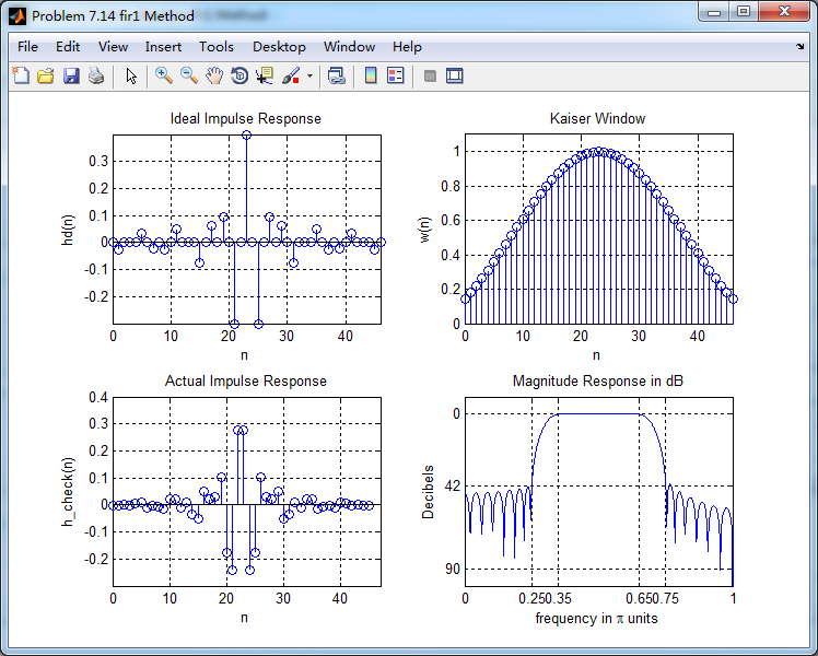
figure('NumberTitle', 'off', 'Name', 'Problem 7.14 fir1 Method')
set(gcf,'Color','white'); 

subplot(2,2,1); stem(n, hd); axis([0 M-1 -0.3 0.4]); grid on;
xlabel('n'); ylabel('hd(n)'); title('Ideal Impulse Response');

subplot(2,2,2); stem(n, w_kai); axis([0 M-1 0 1.1]); grid on;
xlabel('n'); ylabel('w(n)'); title('Kaiser Window');

subplot(2,2,3); stem([0:N], h_check); axis([0 M -0.3 0.4]); grid on;
xlabel('n'); ylabel('h\_check(n)'); title('Actual Impulse Response');

subplot(2,2,4); plot(w/pi, db); axis([0 1 -100 10]); grid on;
set(gca,'YTickMode','manual','YTick',[-90,-42,0]);
set(gca,'YTickLabelMode','manual','YTickLabel',['90';'42';' 0']);
set(gca,'XTickMode','manual','XTick',[0,f,1]);
xlabel('frequency in pi units'); ylabel('Decibels'); title('Magnitude Response in dB');


figure('NumberTitle', 'off', 'Name', 'Problem 7.14 h_check(n) fir1 Method')
set(gcf,'Color','white'); 

subplot(2,2,1); plot(w/pi, db); grid on; axis([0 2 -100 10]); 
xlabel('frequency in pi units'); ylabel('Decibels'); title('Magnitude Response in dB');
set(gca,'YTickMode','manual','YTick',[-90,-42,0])
set(gca,'YTickLabelMode','manual','YTickLabel',['90';'42';' 0']);
set(gca,'XTickMode','manual','XTick',[0,f,1+f,2]);

subplot(2,2,3); plot(w/pi, mag); grid on; %axis([0 2 -100 10]); 
xlabel('frequency in pi units'); ylabel('Absolute'); title('Magnitude Response in absolute');
set(gca,'XTickMode','manual','XTick',[0,f,1+f,2]);
set(gca,'YTickMode','manual','YTick',[0,0.5, 1])

subplot(2,2,2); plot(w/pi, pha); grid on; %axis([0 1 -100 10]); 
xlabel('frequency in pi units'); ylabel('Rad'); title('Phase Response in Radians');
subplot(2,2,4); plot(w/pi, grd*pi/180);  grid on; %axis([0 1 -100 10]); 
xlabel('frequency in pi units'); ylabel('Rad'); title('Group Delay');

　　运行结果：

        使用fir1函数得到的对应结果