原文链接 小样本学习与智能前沿 。 在这个公众号后台回复“200527”,即可获得课件电子资源。

Few-shot image classification
Three regimes of image classification

Problem formulation
Training set consists of labeled samples from lots of “tasks”, e.g., classifying cars, cats, dogs, planes . . .
Data from the new task, e.g., classifying strawberries has:

Few-shot setting considers the case when s is small.
A flavor of current few-shot algorithms
Meta-learning forms the basis for almost all current algorithms. Here’s one successful instantiation.
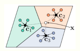
Prototypical Networks [Snell et al., 2017]
- Collect a meta-training set, this consists of a large number of related tasks
- Train one model on all these tasks to ensure that the clustering of features of this model correctly classifies the task
- If the test task comes from the same distribution as the meta-training tasks, we can use the clustering on the new task to classify new classes

How well does few-shot learning work today?

The key idea
A classifier trained on a dataset (D_s) is a function F that classifies data x using

The parameters (θ^∗ = θ(D_s )) of the classifier are a statistic of the dataset Ds obtained after training. Maintaining this statistic avoids having to search over functions F at inference time.
We cannot learn a good (sufficient) statistic using few samples. So we will search over functions at test-time more explicitly

Transductive Learning
 ## A very simple baseline
- Train a large deep network on the meta-training dataset with the standard classification loss
- Initialize a new “classifier head” on top of the logits to handle new classes
- Fine-tune with the few labeled data from the new task
- Perform transductive learning using the unlabeled test data
with a few practical tricks like cosine annealing of step-sizes,
mixup regularization, 16-bit training, very heavy data augmentation, and label smoothing cross-entrop
An example

Results on benchmark datasets

The ImageNet-21k dataset

1-shot, 5-way accuracies are as high as 89%, 1-shot 20-way accuracies are about 70%.
A proposal for systematic evaluation

A thermodynamical view of representation learning
表征学习的热力学观点
Transfer learning
Let’s take an example from computer vision
(.Zamir, A. R., Sax, A., Shen, W., Guibas, L. J., Malik, J., & Savarese, S. Taskonomy: Disentangling task transfer learning. CVPR 2018)

Information Bottleneck Principle
信息瓶颈原则
A generalization of rate-distortion theory for learning relevant representations of data [Tishby et al., 2000]

Z is a representation of the data X. We want
- Z to be sufficient to predict the target Y , and
- Z to be small in size, e.g., few number of bits.

Doing well on one task requires throwing away nuisance information [Achille & Soatto, 2017].
The key idea
The IB Lagrangian simply minimizes (I(X;Z)), it does not let us measure what was thrown away.
Choose a canonical task to measure discarded information. Setting

i.e., reconstruction of data, gives a special task. It is the superset of all tasks and forces the model to learn lossless representations.
The architecture we will focus on is

An auto-encoder
Shanon entropy measures the complexity of data

Distortion D measures the quality of reconstruction

Rate R measures the average excess bits used to encode the representation

Rate-Distortion curve
We know that [Alemi et al., 2017]

this is the well-known ELBO (evidence lower-bound). Let

This is a Lagrange relaxation of the fact that given a variational family and data there is an optimal value R = func(D) that best sandwiches (1).

Rate-Distortion-Classification (RDC) surface
Let us extend the Lagrangian to

where the classification loss is

Can also include other quantities like the entropy S of the model parameters


The existence of a convex surface func(R,D,C,S) = 0 tying together these functionals allows a formal connection to thermodynamics [Alemi and Fischer 2018]

Just like energy is conserved in physical processes, information is conserved in the model, either it is in the encoder-classifier pair or it is in the decoder.
Equilibrium surface of optimal free-energy
The RDC surface determines all possible representations that can be learnt from given data. Can solve the variational problem for F(λ,γ) to get

and

This is called the “equilibrium surface” because training converges to some point on this surface. We now construct ways to travel on the surface
 The surface depends on data p(x,y).
An iso-classification loss process
A quasi-static process happens slowly enough for the system to remain in equilibrium with its surroundings, e.g., reversible expansion of an ideal gas.
We will create a quasi-static process to travel on the RDC surface. This constraint is

e.g., if we want classification loss to be constant in time, we need

……
更多精彩,请下载 资源文件 了解。
关注公众号“小样本学习与智能前沿”,回台回复“200527” ,即可获取资源文件“Learning with Few Labeled Data.pdf”

Summary
Simple methods such as transductive fine-tuning work extremely well for few-shot learning. This is really because of powerful function approximators such as neural networks.
The RDC surface is a fundamental quantity and enables principled methods for transfer learning. Also unlocks new paths to understanding regularization and properties of neural architecture for classical supervised learning.
We did well in the era of big data without understanding much about data; this is unlikely to work in the age of little data.
Email questions to pratikac@seas.upenn.edu Read more at
- Dhillon, G., Chaudhari, P., Ravichandran, A., and Soatto, S. (2019). A baseline for few-shot image classification. arXiv:1909.02729. ICLR 2020.
- Li, H., Chaudhari, P., Yang, H., Lam, M., Ravichandran, A., Bhotika, R., & Soatto, S. (2020). Rethinking the Hyperparameters for Fine-tuning. arXiv:2002.11770. ICLR 2020.
- Fakoor, R., Chaudhari, P., Soatto, S., & Smola, A. J. (2019). Meta-Q-Learning. arXiv:1910.00125. ICLR 2020.
- Gao, Y., and Chaudhari, P. (2020). A free-energy principle for representation learning. arXiv:2002.12406.