用python实习逻辑回归

建立一个逻辑回归模型来预测一个学生是否被大学录取

# 三大件
import numpy as np
import pandas as pd
import matplotlib.pyplot as plt

import os
path = 'data' + os.sep + 'LogiReg_data.txt'
pdData = pd.read_csv(path, header=None, names=['Exam1', 'Exam2', 'Admitted'])
print(pdData.head())
# 看一下数据的维度
print(pdData.shape)
# 画图看一下每一个为 0 的数量和为 1 的数量
positive = pdData[pdData['Admitted'] == 1]
negative = pdData[pdData['Admitted'] == 0]

fig, ax = plt.subplots(figsize=(10, 5))
ax.scatter(positive['Exam1'], positive['Exam2'], s=30, c='b', marker='o', label='Admitted')
ax.scatter(negative['Exam1'], negative['Exam2'], s=30, c='r', marker='x', label='Not Admitted')
ax.legend()
ax.set_xlabel('Exam1 Score')
ax.set_ylabel('Exam2 Score')

plt.show()


# 逻辑回归
# 目标: 建立分类器(求解出三个参数)
# 设定阀值, 根据阀值判断录取结果 - 0.5

# 要完成的模块
# sigmoid: 映射到概率的函数
# model:返回预测结果
# cost: 根据参数计算损失
# gradient:计算每个参数的梯度方向
# descent: 进行参数更新
# accuracy: 计算精度

# sigmoid函数 g(x)
def sigmoid(z):
    return 1 / (1 + np.exp(-z))
# sigmoid 函数画图
# nums = np.linspace(-10, 10, 100)
# fig, ax = plt.subplots(figsize=(12, 4))
# ax.plot(nums, sigmoid(nums))
# plt.show()
# 建立模型, 这个是预测函数, h(x) = g(z)

def model(X, theta):
    return sigmoid(np.dot(X, theta.T))

# 因为参数是三个, 所以添加一列
pdData.insert(0, 'Ones', 1)
print(pdData.head())
# 设置X(training data) 和 y(target)
orig_date = pdData.values
cols = orig_date.shape[1]
print(cols)
X = orig_date[:, 0:cols-1]
y = orig_date[:,cols-1:cols]
print(X[:5])
print(y[:5])

theta = np.zeros([1, 3])
print(theta)
print(X.shape)
print(y.shape)
print(theta.shape)

# 损失函数

def cost(X, y, theta):
    left = np.multiply(-y, np.log(model(X, theta)))
    right = np.multiply(1-y, np.log(1 - model(X,theta)))
    return np.sum(left - right) / len(X)

print(cost(X, y, theta))

# 计算梯度

def gradient(X, y, theta):
    grad = np.zeros(theta.shape)
    error = (model(X, theta) - y).ravel()
    for j in range(len(theta.ravel())): # for each parmeter
        term = np.multiply(error, X[:, j])
        grad[0, j] = np.sum(term) / len(X)

    return grad

# Gradient Descent
# 比较3种不同梯度下降的方法

STOP_ITER = 0  # 迭代次数, 比如2000
STOP_COST = 1  # 根据两次迭代损失值变化, 差异比较小
STOP_GRAD = 2  # 根据梯度, 两次梯度差不多, 没啥变化
# 模型优化, 停止策略

def stopCriterion(type, value, threshold):
    # 设定三种不同的停止策略
    if type == STOP_ITER: return value > threshold
    elif type == STOP_COST: return abs(value[-1]- value[-2]) < threshold
    elif type == STOP_GRAD: return np.linalg.norm(value) < threshold

# 对数据进行洗牌
import numpy.random

def shuffleData(data):
    np.random.shuffle(data)
    cols = data.shape[1]
    X = data[:, 0:cols-1]
    y = data[:, cols-1:]
    return X, y


import time

# 看时间对结果的影响
def descent(data, theta, batchSize, stopType, thresh, alpha):
    # 梯度下降求解
    init_time = time.time()
    i = 0 # 迭代次数
    k = 0 # batch
    X, y = shuffleData(data)
    grad = np.zeros(theta.shape) # 计算梯度
    costs = [cost(X, y, theta)] # 损失值
    i += 1
    n = len(data)
    while True:
        grad  = gradient(X[k:k+batchSize], y[k:k+batchSize], theta)
        k += batchSize # 取batch数量个数据
        if k >= n:
            k = 0
            X, y = shuffleData(data) # 重新洗牌
        theta = theta - alpha*grad # 参数更新
        costs.append(cost(X, y, theta))

        i += 1

        if stopType == STOP_ITER: value = i
        elif stopType == STOP_COST: value = costs
        elif stopType == STOP_GRAD: value = grad
        if stopCriterion(stopType, value, thresh): break

    return theta, i-1, costs, grad, time.time()-init_time


def runExpe(data, theta, batchSize, stopType, thresh, alpha):
    # import pdb
    theta, iter, costs, grad, dur = descent(data, theta, batchSize, stopType, thresh, alpha)
    name = 'Original' if (data[:, 1] > 2).sum() > 1 else 'Scaled'
    name += " data - learning rate :{} - ".format(alpha)
    n = len(data)
    if batchSize == n: strDescType = "Gradient"
    elif batchSize == 1: strDescType = 'SGD'
    else: strDescType = 'Mini-batch({})'.format(batchSize)

    name += strDescType + " descent - Stop: "
    if stopType == STOP_ITER: strStop = "{} iterations".format(thresh)
    elif stopType == STOP_COST: strStop = 'costs change < {}'.format(thresh)
    else: strStop = "gradient norm < {}".format(thresh)
    name += strStop
    print("***{}
Theta: {} - Iter: {} - Last cost: {:03.2f} - Duration:{:03.2f}s".format(name, theta, iter, costs[-1], dur))
    fig, ax = plt.subplots(figsize=(12, 4))
    ax.plot(np.arange(len(costs)), costs, 'r')
    ax.set_xlabel('Iterations')
    ax.set_ylabel('Cost')
    ax.set_title(name.upper() + ' - Error vs Iteration')
    plt.show()
    return theta

# 选择的梯度下降方法是基于所有样本的
n = 100
# runExpe(orig_date, theta, n, STOP_ITER, thresh=5000, alpha=0.000001)


# 根据阀值进行1E-6 差不多需要110 000次迭代
# runExpe(orig_date, theta, n, STOP_COST, thresh=0.000001, alpha=0.001)

# 对比不同的梯度下降方法
# Stochastic descent
# runExpe(orig_date, theta, 1, STOP_ITER, thresh=5000, alpha=0.001)
# 有点爆炸,很不稳定, 再来试试把学习率调小一点
# runExpe(orig_date, theta, 1, STOP_ITER, thresh=5000, alpha=0.000002)

# 速度快,但是稳定性查, 需要哦很小的学习率
# Mini-batch descent
# runExpe(orig_date, theta, 16, STOP_ITER, thresh=15000, alpha=0.00001)


# 浮动比较大, 我们来尝试对数据进行标准化, 将数据按属性值减去其均值,然后除以方差, 最后得到的结果是,对每个属性/每列均值都在0附近,方差为1
from sklearn import preprocessing as pp

scaled_data = orig_date.copy()
scaled_data[:, 1:3] = pp.scale(orig_date[:, 1:3])
print(scaled_data)

# runExpe(scaled_data, theta, n, STOP_ITER, thresh=5000, alpha=0.001)

# 先改数据,再改模型

# runExpe(scaled_data, theta, n, STOP_GRAD, thresh=0.02, alpha=0.001)

# 它好多了, 原始数据, 只能达到0.61, 而我们得到了0.38在这里, 所以做数据预处理是非常重要的

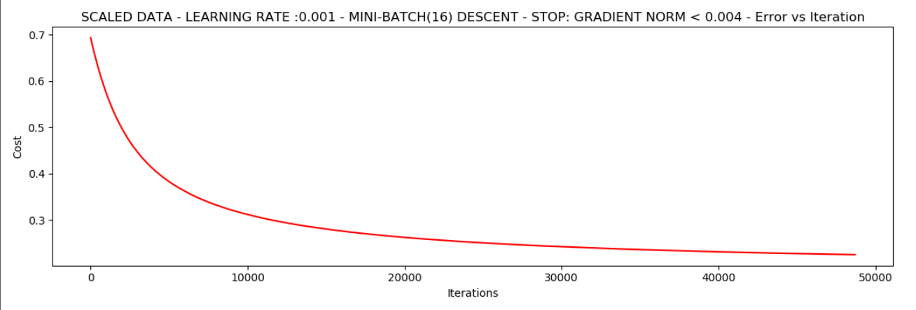
runExpe(scaled_data, theta, 16, STOP_GRAD, thresh=0.002*2, alpha=0.001)
# 精度
# 设定阀值
def predict(X, theta):
    return [1 if x > 0.5 else 0 for x in model(X, theta)]

#
scaled_X = scaled_data[:, :3]
y = scaled_data[:, 3]
predictions = predict(scaled_X, theta)

correct = [1 if ((a == 1 and b == 1) or (a == 0 and b == 0)) else 0 for (a, b) in zip(predictions, y)]
print(len(correct))

accuracy = (sum(map(int, correct)) % len(correct))
print("accuracy = {0}%".format(accuracy))

最后的损失函数

------------恢复内容结束------------