metrics是sklearn用来做模型评估的重要模块,提供了各种评估度量,现在自己整理如下:
一.通用的用法:Common cases: predefined values
1.1 sklearn官网上给出的指标如下图所示:
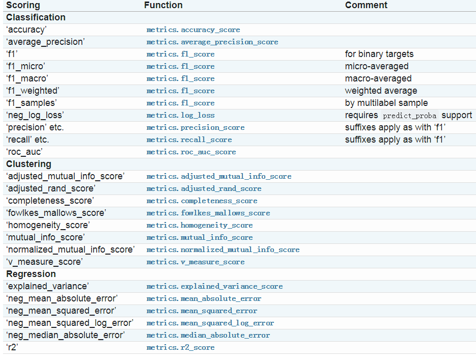
1.2除了上图中的度量指标以外,你还可以自定义一些度量指标:通过sklearn.metrics.make_scorer()方法进行定义;
make_scorer有两种典型的用法:
用法一:包装一些在metrics中已经存在的的方法,但是这种方法需要一些参数,例如fbeta_score方法,官网上给出的用法如下:
from sklearn.metrics import fbeta_score, make_scorer
ftwo_scorer = make_scorer(fbeta_score, beta=2)
from sklearn.model_selection import GridSearchCV
from sklearn.svm import LinearSVC
grid = GridSearchCV(LinearSVC(), param_grid={'C': [1, 10]}, scoring=ftwo_scorer)
第二种用法是完全的定义用户自定义的函数,可以接受一下几种参数:
1.你想用的python函数;
2、不论你提供的python函数返回的是socre或者是loss,if score:the higher the better;if loss: the lower the better
3、只为分类度量:无论你提供的python方法是不是需要连续的决策因素,默认为否
4.其他额外的参数,例如f1_score中的beta或者labels
例如官网上给出的例子:
import numpy as np
def my_custom_loss_func(ground_truth, predictions):
    diff = np.abs(ground_truth - predictions).max()
    return np.log(1 + diff)

# loss_func will negate the return value of my_custom_loss_func,
#  which will be np.log(2), 0.693, given the values for ground_truth
#  and predictions defined below.
loss  = make_scorer(my_custom_loss_func, greater_is_better=False)
score = make_scorer(my_custom_loss_func, greater_is_better=True)
ground_truth = [[1], [1]]
predictions  = [0, 1]
from sklearn.dummy import DummyClassifier
clf = DummyClassifier(strategy='most_frequent', random_state=0)
clf = clf.fit(ground_truth, predictions)
loss(clf,ground_truth, predictions)
-0.69...
score(clf,ground_truth, predictions)
0.69...
1.3 使用多重度量标准
sklearn也接受在GridSearchCV,RandomizedSearchCV和Cross_validate中接受多指标,有两种指定方式;
##方式1: 使用字符串的list
scoring=['accuracy','precision']

### f方式2:使用dict进行mapping
from sklearn.metrics import accuracy_score
from sklearn.metrics import make_scorer
scoring = {'accuracy': make_scorer(accuracy_score),
           'prec': 'precision'}
注意:目前方式2(dict)模式只允许返回单一score的score方法,返回多个的需要进行加工处理,例如官方上给出的加工处理混淆矩阵的方法:
from sklearn.model_selection import cross_validate
from sklearn.metrics import confusion_matrix
# A sample toy binary classification dataset
X, y = datasets.make_classification(n_classes=2, random_state=0)
svm = LinearSVC(random_state=0)
def tp(y_true, y_pred): return confusion_matrix(y_true, y_pred)[0, 0]
def tn(y_true, y_pred): return confusion_matrix(y_true, y_pred)[0, 0]
def fp(y_true, y_pred): return confusion_matrix(y_true, y_pred)[1, 0]
def fn(y_true, y_pred): return confusion_matrix(y_true, y_pred)[0, 1]
scoring = {'tp' : make_scorer(tp), 'tn' : make_scorer(tn),
           'fp' : make_scorer(fp), 'fn' : make_scorer(fn)}
cv_results = cross_validate(svm.fit(X, y), X, y, scoring=scoring)
# Getting the test set true positive scores
print(cv_results['test_tp'])
[12 13 15]
# Getting the test set false negative scores
print(cv_results['test_fn'])
[5,4,1]
二:分类指标;
针对分类,sklearn也提供了大量的度量指标,而且针对不同的分类(二分类,多分类,)有不同的度量指标,官网截图如下:
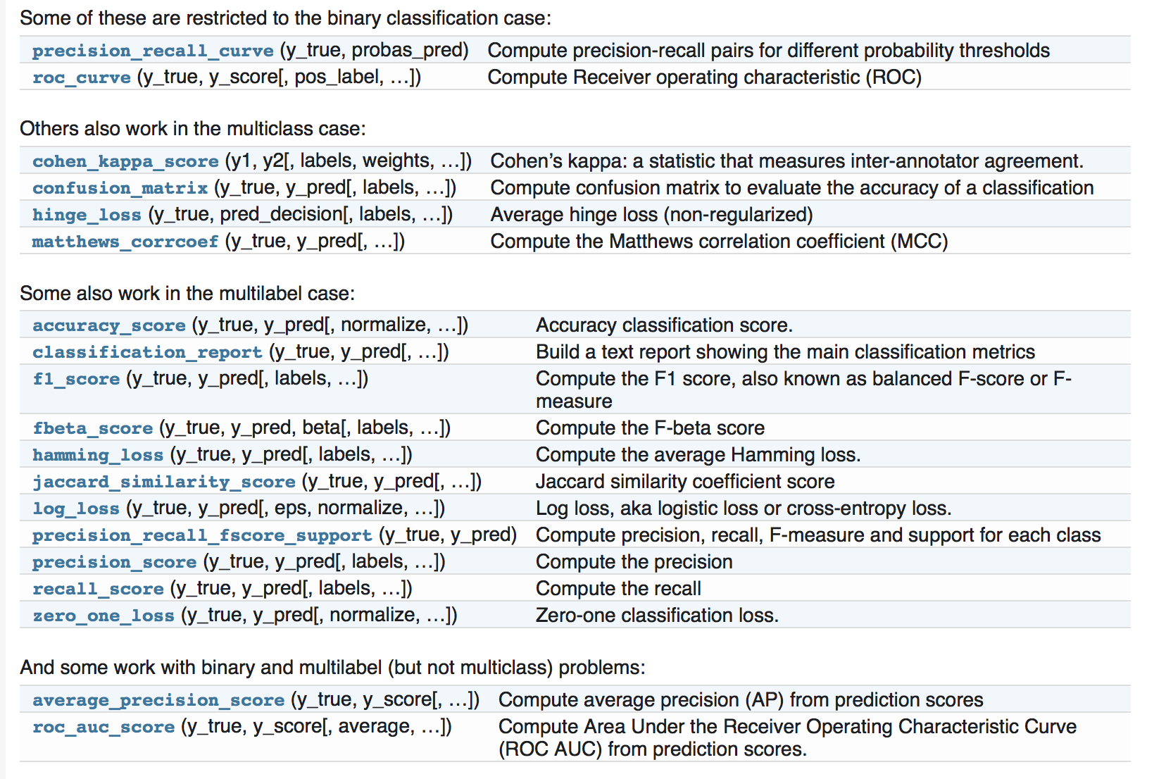
2.1 从二分类到多分类问题:
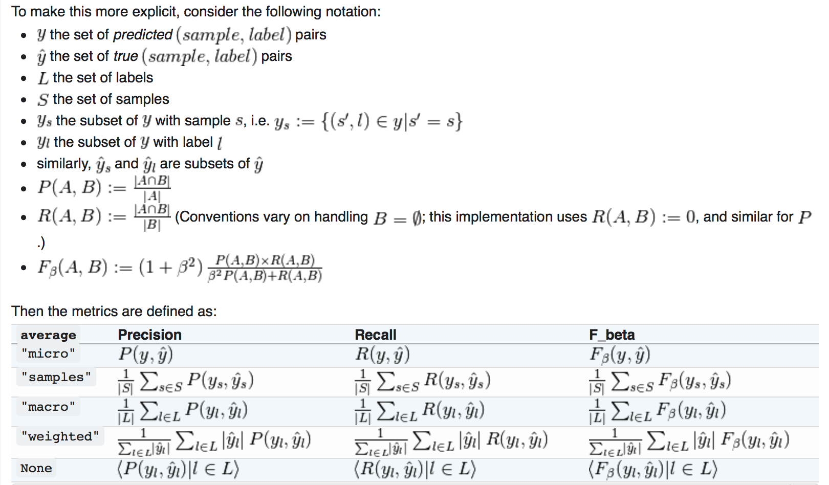
像f1_score, roc_auc_score这种度量指标大多是针对二分类问题的,但是为了将二分类的度量指标延伸到多分类问题,数据将会看做是二分类问题的集合,也就是1vs all;有好几种方式来平衡不同类别的二分度量,通过使用average参数来进行设置。
(1)marco(宏平均):当频繁的类别非常重要时,宏平均可以会突出他的性能表现;当然所有的类别同样重要是不现实的,因此宏平均可能会过度强调低频繁类别的低性能表现;
(2)weighted(权重)
(3)micro(微平均):微平均可能在多标签的分类问题的首选
(4)samples(样本):仅仅当多标签问题是可以采用。
多分类问题转换到二分类问题就是采用1vs all的方式;
2.2 准确率(accuracy)
采用accuracy_score来计算模型的accuracy,计算公式如下:
 ,其中
,其中 表示预测y值,yi表示实际的y值;
##
import numpy as np
from sklearn.metrics import accuracy_score
y_pred = [0, 2, 1, 3]
y_true = [0, 1, 2, 3]
accuracy_score(y_true, y_pred)
0.5
accuracy_score(y_true, y_pred, normalize=False)
2
###多分类问题
accuracy_score(np.array([[0, 1], [1, 1]]), np.ones((2, 2)))
0.5
2.3混淆矩阵
混淆矩阵是评价分类问题的一个典型度量,在sklearn中使用 confusion_matrix;
from sklearn.metrics import confusion_matrix
y_true = [2, 0, 2, 2, 0, 1]
y_pred = [0, 0, 2, 2, 0, 2]
confusion_matrix(y_true, y_pred)
array([[2, 0, 0],
       [0, 0, 1],
       [1, 0, 2]])
混淆矩阵Rij(多分类)的含义表示类别i被预测成类别j的次数,因此Rii表示被正确分类的次数;
对于二分类问题,混淆矩阵用来表示TN,TP,FN,FP;
y_true = [0, 0, 0, 1, 1, 1, 1, 1]
y_pred = [0, 1, 0, 1, 0, 1, 0, 1]
tn, fp, fn, tp = confusion_matrix(y_true, y_pred).ravel()
tn, fp, fn, tp
(2, 1, 2, 3)
官网上提供的混淆矩阵的可视化例子:http://scikit-learn.org/stable/auto_examples/model_selection/plot_confusion_matrix.html#sphx-glr-auto-examples-model-selection-plot-confusion-matrix-py
2.4 Classification report
Classification report展示了分类的主要度量指标,如下面例子所示:
from sklearn.metrics import classification_report
y_true = [0, 1, 2, 2, 0]
y_pred = [0, 0, 2, 1, 0]
target_names = ['class 0', 'class 1', 'class 2']
print(classification_report(y_true, y_pred, target_names=target_names))
             precision    recall  f1-score   support

    class 0       0.67      1.00      0.80         2
    class 1       0.00      0.00      0.00         1
    class 2       1.00      0.50      0.67         2

avg / total       0.67      0.60      0.59         5
2.5 Hamming loss
Hamming loss计算预测结果和实际结果的海明距离,计算公式如下:
 ,简单的理解就是预测样本中误差总数除以样本总数
例子:
from sklearn.metrics import hamming_loss
y_pred = [1, 2, 3, 4]
y_true = [2, 2, 3, 4]
hamming_loss(y_true, y_pred)
0.25
##在多标签分类中同样适合
hamming_loss(np.array([[0, 1], [1, 1]]), np.zeros((2, 2)))
0.75
2.6 Jaccard 相关系数:
Jaccard相关系数在推荐系统中经常使用,可以理解为预测正确的个数除以总的样本数,所以在二分类问题中,Jaccard系数和准确率是一样的。
 ,
,
例子:
import numpy as np
from sklearn.metrics import jaccard_similarity_score
y_pred = [0, 2, 1, 3]
y_true = [0, 1, 2, 3]
jaccard_similarity_score(y_true, y_pred)
0.5
jaccard_similarity_score(y_true, y_pred, normalize=False)
2
##multilabel
jaccard_similarity_score(np.array([[0, 1], [1, 1]]), np.ones((2, 2)))
0.75
2.7 precision,召回率,F系数等
(1)精准率(precision):正确预测为正例的样本数占全部预测为正例的样本数的比例;
(2)召回率:正例样本中预测正确的样本占实际正例样本数量的比例;
(3)F系数同时兼顾了分类模型的准确率和召回率。F1分数可以看作是模型准确率和召回率的一种加权平均,它的最大值是1,最小值是0。
计算公式:
分数为
precision_recall_curve:准确率召回率曲线 ,其中where
  and
and  are the precision and recall at the nth threshold.


>>> from sklearn import metrics
>>> y_pred = [0, 1, 0, 0]
>>> y_true = [0, 1, 0, 1]
>>> metrics.precision_score(y_true, y_pred)
1.0
>>> metrics.recall_score(y_true, y_pred)
0.5
>>> metrics.f1_score(y_true, y_pred)
0.66...
>>> metrics.fbeta_score(y_true, y_pred, beta=0.5)
0.83...
>>> metrics.fbeta_score(y_true, y_pred, beta=1)
0.66...
>>> metrics.fbeta_score(y_true, y_pred, beta=2)
0.55...
>>> metrics.precision_recall_fscore_support(y_true, y_pred, beta=0.5)
(array([ 0.66...,  1.        ]), array([ 1. ,  0.5]), array([ 0.71...,  0.83...]), array([2, 2]...))


>>> import numpy as np
>>> from sklearn.metrics import precision_recall_curve
>>> from sklearn.metrics import average_precision_score
>>> y_true = np.array([0, 0, 1, 1])
>>> y_scores = np.array([0.1, 0.4, 0.35, 0.8])
>>> precision, recall, threshold = precision_recall_curve(y_true, y_scores)
>>> precision
array([ 0.66...,  0.5       ,  1.        ,  1.        ])
>>> recall
array([ 1. ,  0.5,  0.5,  0. ])
>>> threshold
array([ 0.35,  0.4 ,  0.8 ])
>>> average_precision_score(y_true, y_scores)
0.83...
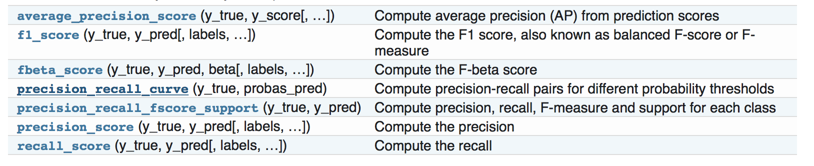
对于多类别分类和多标签分类,同样提供的一样的评价指标;
例子:
>>> from sklearn import metrics
>>> y_true = [0, 1, 2, 0, 1, 2]
>>> y_pred = [0, 2, 1, 0, 0, 1]
>>> metrics.precision_score(y_true, y_pred, average='macro')
0.22...
>>> metrics.recall_score(y_true, y_pred, average='micro')
...
0.33...
>>> metrics.f1_score(y_true, y_pred, average='weighted')
0.26...
>>> metrics.fbeta_score(y_true, y_pred, average='macro', beta=0.5)
0.23...
>>> metrics.precision_recall_fscore_support(y_true, y_pred, beta=0.5, average=None)
...
(array([ 0.66...,  0.        ,  0.        ]), array([ 1.,  0.,  0.]), array([ 0.71...,  0.        ,  0.        ]), array([2, 2, 2]...))
2.8 ROC曲线
ROC曲线是建模结果比较熟悉的一中展示方式:
例如如下代码:
import numpy as np
from sklearn.metrics import roc_curve
from sklearn.datasets import load_iris
from sklearn import svm
from sklearn.linear_model import LogisticRegression
from sklearn.cross_validation import train_test_split
from sklearn.metrics import roc_auc_score
from sklearn.metrics import roc_curve
import matplotlib.pyplot as plt

data=load_iris()
###两分类
X,y=data.data,data.target


X_train,X_test,y_train,y_test=train_test_split(X,y)
est=svm.SVC(probability=True)
model=est.fit(X_train,y_train)
y_score=model.decision_function(X_test)
fpr1,tpr1,thresholds1=roc_curve(y_test,model.predict_proba(X_test)[:,1],pos_label=1)

lr=LogisticRegression()
lr.fit(X_train,y_train)
fpr2,tpr2,thresholds2=roc_curve(y_test,lr.predict_proba(X_test)[:,1],pos_label=1)

plt.plot(fpr1,tpr1,linewidth=1,label='ROC of svm')
plt.plot(fpr2,tpr2,linewidth=1,label='ROC of LR')
plt.xlabel('FPR')
plt.ylabel('TPR')
plt.plot([0,1],[0,1],linestyle='--')
plt.legend(loc=4)
plt.show()

结果如上图所示。