PCA算法数学原理及实现

数学原理参考：https://blog.csdn.net/aiaiai010101/article/details/72744713

实现过程参考：https://www.cnblogs.com/eczhou/p/5435425.html

两篇博文都写的透彻明白。

自己用python实现了一下，有几点疑问，主要是因为对基变换和坐标变换理解不深。

先附上代码和实验结果：

code：

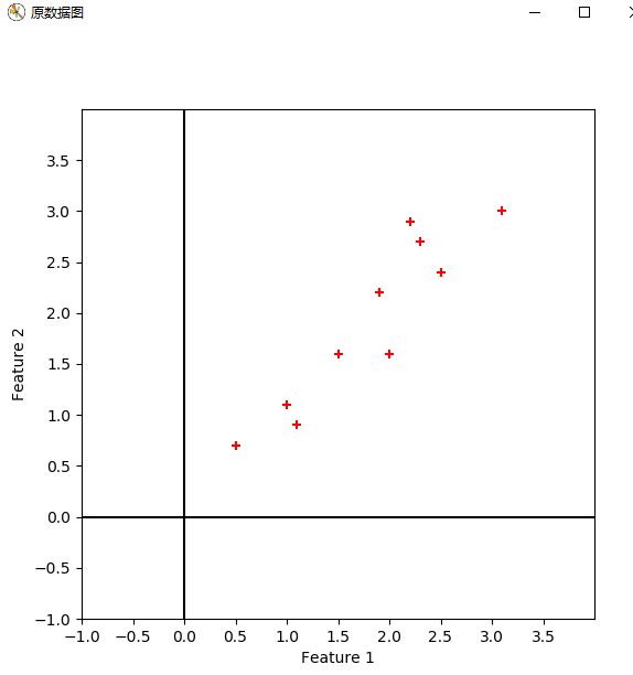
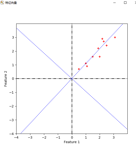
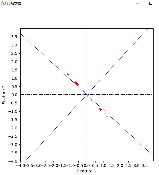
from numpy import *
import numpy as np
import matplotlib.pyplot as plt
from scipy.io import loadmat

cx = mat([[2.5, 2.4],
          [0.5, 0.7],
          [2.2, 2.9],
          [1.9, 2.2],
          [3.1, 3.0],
          [2.3, 2.7],
          [2, 1.6],
          [1, 1.1],
          [1.5, 1.6],
          [1.1, 0.9]])
# print(cx.shape)
sz = cx.shape
m = sz[0]
n = sz[1]

# 显示原数据
def plot_oridata( cx ):
    plt.figure(num='原数据图', figsize=(6, 6))
    plt.xlabel('Feature 1')
    plt.ylabel('Feature 2')
    plt.xlim((-1, 4))
    plt.ylim((-1, 4))
    new_ticks = np.arange(-1, 4, 0.5)
    plt.xticks(new_ticks)
    plt.yticks(new_ticks)
    plt.scatter(cx[:, 0].tolist(), cx[:, 1].tolist(), c='r', marker='+')
    plt.plot([0, 0], [-1, 4], 'k-')
    plt.plot([-1, 4], [0, 0], 'k-')
    plt.show()
    return

#求协方差矩阵
def get_covMat( cx ):
    print('+++++++++++++       求协方差矩阵     +++++++++++++++')
    # 零均值化
    ecol = np.mean(cx, axis=0)
    cx1 = (cx[:, 0]) - ecol[0, 0]
    cx2 = cx[:, 1] - ecol[0, 1]
    Mcx = np.column_stack((cx1, cx2))
    Covx = np.transpose(Mcx)*Mcx/(m-1)
    # print(Covx)
    return Covx, Mcx

#计算特征值和特征向量
def get_eign(Covx, k):
    eVals, eVecs = np.linalg.eig(Covx)
    # print(eVals)
    # print(eVecs, ' ', eVecs.shape)
    sorted_indices = np.argsort(eVals)
    topk_evecs = eVecs[:, sorted_indices[:-k-1:-1]]
    # print(topk_evecs)

    plt.figure(num='特征向量', figsize=(6, 6))
    plt.xlabel('Feature 1')
    plt.ylabel('Feature 2')
    plt.xlim((-4, 4))
    plt.ylim((-4, 4))
    new_ticks = np.arange(-4, 4, 1)
    plt.xticks(new_ticks)
    plt.yticks(new_ticks)
    plt.scatter(cx[:, 0].tolist(), cx[:, 1].tolist(), c='r', marker='+')
    plt.plot([0, 0], [-4, 4], 'k-.')
    plt.plot([-4, 4], [0, 0], 'k-.')
    # print(eVecs[0, 0], eVecs[1, 0])
    # print(eVecs)
    plt.plot([0, eVecs[0, 0] * 6], [0, eVecs[1, 0] * 6], 'b:')
    plt.plot([0, eVecs[0, 1] * 6], [0, eVecs[1, 1] * 6], 'b:')
    plt.plot([0, eVecs[0, 0] * -6], [0, eVecs[1, 0] * -6], 'b:')
    plt.plot([0, eVecs[0, 1] * -6], [0, eVecs[1, 1] * -6], 'b:')
    plt.show()
    return eVecs, topk_evecs

#转换数据
def transform_data(eVecs, Mcx):
    print("------------------转换数据---------------------")
    tran_data = Mcx * eVecs
    plt.figure(num='转换数据', figsize=(6, 6))
    plt.xlabel('Feature 1')
    plt.ylabel('Feature 2')
    plt.xlim((-2, 2))
    plt.ylim((-2, 2))
    new_ticks = np.arange(-2, 2, 0.5)
    plt.xticks(new_ticks)
    plt.yticks(new_ticks)
    plt.scatter(tran_data[:, 0].tolist(), tran_data[:, 1].tolist(), c='r', marker='+')#哪一维对应x,哪一维对应y
    plt.plot([0, 0], [-4, 4], 'k-.')
    plt.plot([-4, 4], [0, 0], 'k-.')
    # print(eVecs[0, 0], eVecs[1, 0])
    # print(eVecs)
    plt.show()
    return

#压缩数据
def compress_data(Mcx, topkevecs, eVecs):
    print("------------------压缩数据---------------------")
    comdata = Mcx * topkevecs
    c1 = np.zeros((10, 1), dtype=int)
    comdata1 = np.column_stack((c1, comdata))
    comdata2 = comdata1 * eVecs

    plt.figure(num='压缩数据', figsize=(6, 6))
    plt.xlabel('Feature 1')
    plt.ylabel('Feature 2')
    plt.xlim((-4, 4))
    plt.ylim((-4, 4))
    new_ticks = np.arange(-4, 4, 0.5)
    plt.xticks(new_ticks)
    plt.yticks(new_ticks)
    plt.scatter(comdata2[:, 0].tolist(), comdata2[:, 1].tolist(), c='r', marker='+')  # 哪一维对应x,哪一维对应y
    plt.plot([0, 0], [-4, 4], 'k-.')
    plt.plot([-4, 4], [0, 0], 'k-.')
    plt.plot([0, eVecs[0, 0] * 6], [0, eVecs[1, 0] * 6], 'b:')
    plt.plot([0, eVecs[0, 1] * 6], [0, eVecs[1, 1] * 6], 'b:')
    plt.plot([0, eVecs[0, 0] * -6], [0, eVecs[1, 0] * -6], 'b:')
    plt.plot([0, eVecs[0, 1] * -6], [0, eVecs[1, 1] * -6], 'b:')
    # print(eVecs[0, 0], eVecs[1, 0])
    # print(eVecs)
    plt.show()
    return

plot_oridata(cx)
Covx, Mcx = get_covMat(cx)
eVecs, topk_evecs = get_eign(Covx, 1)
transform_data(eVecs, Mcx)
compress_data(Mcx, topk_evecs, eVecs)
print('end')

初学python，代码肯定很啰嗦，并且很丑。

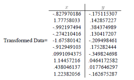
实验结果：

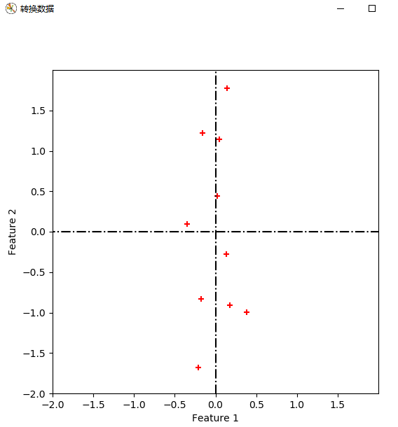
疑问1：对数据进行特征向量为基的转换时，公式如下。我得到的坐标是以原坐标系为参考的，那么哪一维对应x，哪一维对应y，如果我将特征向量按照特征值降序的顺序重新排列，是否有影响呢？

得到的坐标是新坐标系下的。根据转换向量对应。

            

疑问2：取最大特征值对应的特征向量为基时，对数据进行降维，此时我得到的一维坐标是以这个特征向量为参考的吗？此时我应该如何在原坐标系show出这些数据？

我的代码中，取第一维为0，第二维为得到的坐标，以此再进行以此疑问1中的二维基转换，得到坐标，并且plot。不太理解道理。

对一维坐标，分别对两个坐标轴投影即可得到新坐标系下的两个坐标。