计算图中的操作
代码实现:
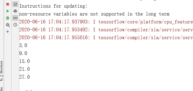
import numpy as np
import tensorflow.compat.v1 as tf
tf.disable_v2_behavior() # 使用静态图模式运行以下代码
assert tf.__version__.startswith('2.')
sess = tf.Session()
x_vals = np.array([1., 3., 5., 7., 9.])
x_data = tf.placeholder(dtype=tf.float32)
m_const = tf.constant(3.)
my_product = tf.multiply(x_data, m_const)
for x_val in x_vals:
    print(sess.run(my_product, feed_dict={x_data:x_val}))
执行结果:
Tensorflow的嵌入Layer
代码实现:
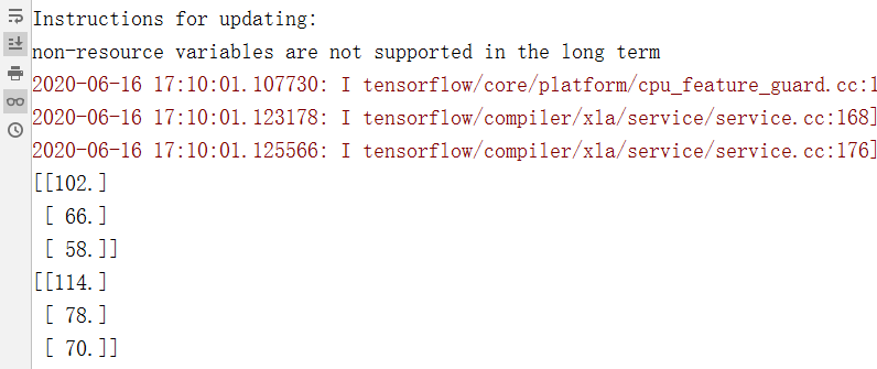
import numpy as np
import tensorflow.compat.v1 as tf
tf.disable_v2_behavior() # 使用静态图模式运行以下代码
assert tf.__version__.startswith('2.')
sess = tf.Session()
# 创建数据和占位符
my_array = np.array([[1., 3., 5., 7., 9.],
                     [-2., 0., 2., 4., 6.],
                     [-6., -3., 0., 3., 6.]])
x_vals = np.array([my_array, my_array+1])
x_data = tf.placeholder(shape=(3,5), dtype=tf.float32)
# 创建常量矩阵
m1 = tf.constant([[1.], [0.], [-1.], [2.], [4.]]) # 5x1矩阵
m2 = tf.constant([[2.]]) # 1x1矩阵
a1 = tf.constant([[10.]]) # 1x1矩阵
# 声明操作, 表示成计算图
prod1 = tf.matmul(x_data, m1) # 3x5 乘以 5x1 = 3x1
prod2 = tf.matmul(prod1, m2) # 3x1 乘以标量 = 3x1
add1 = tf.add(prod2, a1)
# 赋值
for x_val in x_vals:
    print(sess.run(add1, feed_dict={x_data: x_val}))
sess.close()
执行结果:
注意:对于事先不知道的维度大小,可以用None代替。例如:
x_data = tf.placeholder(dtype=tf.float32, shape=(3,None))
Tensorflow的多层layer
对2D图像数据进行滑动窗口平均,然后通过自定义操作层Layer返回结果。
代码实现:
import numpy as np
import tensorflow.compat.v1 as tf
tf.disable_v2_behavior() # 使用静态图模式运行以下代码
assert tf.__version__.startswith('2.')
sess = tf.Session()
# 创建2D图像,4X4像素。
x_shape = [1, 4, 4, 1] # [batch, in_height, in_width, in_channels] tensorflow处理(图片数量,高度、宽度、颜色)思维图像数据
x_val = np.random.uniform(size=x_shape)
# 占位符
x_data = tf.placeholder(dtype=tf.float32, shape=x_shape)
# 创建滑动窗口
my_filter = tf.constant(0.25, shape=[2,2,1,1]) # [filter_height, filter_width, in_channels, out_channels]
my_strides = [1, 2, 2, 1] # 长宽方向滑动步长均为2
mov_avg_layer = tf.nn.conv2d(x_data, my_filter, my_strides,
                            padding='SAME', name='Moving_avg_Window')
# 定义一个自定义Layer,操作上一步滑动窗口的2x2的返回值。
# 自定义函数将输入张量乘以一个2X2的矩阵张量,然后每个元素加1.因为矩阵乘法只计算二维矩阵,所以裁剪多余维度(大小为1的维度)。Tensorflow通过内建函数squeeze()函数裁剪。
def custom_layer(input_matrix):
    input_matrix_squeezed = tf.squeeze(input_matrix)
    A = tf.constant([[1., 2.], [-1., 3.]])
    b = tf.constant(1., shape=[2,2])
    temp1 = tf.matmul(A, input_matrix_squeezed)
    temp = tf.add(temp1, b) # Ax+b
    return (tf.sigmoid(temp))
# 把刚刚定义的Layer加入到计算图中,并用tf.name_scope()命名Layer名称。
with tf.name_scope('Custom_Layer') as scope:
    custom_layer1 = custom_layer(mov_avg_layer)
# 传入数据,执行
print(sess.run(custom_layer1, feed_dict={x_data:x_val}))
# 关闭会话,释放资源
sess.close()
执行结果:

Tensorflow实现损失函数
损失函数对机器学习来讲非常重要,它度量模型输出值与目标值之间的差距。
回归问题常用损失函数
代码实现:
import numpy as np
import matplotlib.pyplot as plt
import tensorflow.compat.v1 as tf
tf.disable_v2_behavior() # 使用静态图模式运行以下代码
assert tf.__version__.startswith('2.')
sess = tf.Session()
# 创建2D图像,4X4像素。
x_shape = [1, 4, 4, 1] # [batch, in_height, in_width, in_channels] tensorflow处理(图片数量,高度、宽度、颜色)思维图像数据
x_val = np.random.uniform(size=x_shape)
# 占位符
x_data = tf.placeholder(dtype=tf.float32, shape=x_shape)
# 创建滑动窗口
my_filter = tf.constant(0.25, shape=[2,2,1,1]) # [filter_height, filter_width, in_channels, out_channels]
my_strides = [1, 2, 2, 1] # 长宽方向滑动步长均为2
mov_avg_layer = tf.nn.conv2d(x_data, my_filter, my_strides,
                            padding='SAME', name='Moving_avg_Window')
# 定义一个自定义Layer,操作上一步滑动窗口的2x2的返回值。
# 自定义函数将输入张量乘以一个2X2的矩阵张量,然后每个元素加1.因为矩阵乘法只计算二维矩阵,所以裁剪多余维度(大小为1的维度)。Tensorflow通过内建函数squeeze()函数裁剪。
def custom_layer(input_matrix):
    input_matrix_squeezed = tf.squeeze(input_matrix)
    A = tf.constant([[1., 2.], [-1., 3.]])
    b = tf.constant(1., shape=[2,2])
    temp1 = tf.matmul(A, input_matrix_squeezed)
    temp = tf.add(temp1, b) # Ax+b
    return (tf.sigmoid(temp))
# 把刚刚定义的Layer加入到计算图中,并用tf.name_scope()命名Layer名称。
with tf.name_scope('Custom_Layer') as scope:
    custom_layer1 = custom_layer(mov_avg_layer)
# 传入数据,执行
print(sess.run(custom_layer1, feed_dict={x_data:x_val}))
# 关闭会话,释放资源
sess.close()
执行结果:

关于Huber函数
L1正则在目标值处不平滑。L2正则在异常值处过大,会放大异常值的影响。因此,Huber函数在目标值附近(小于delta)是L2正则,在大于delta处是L1正则。解决上述问题。
参考
Huber损失函数
绘图展示回归算法损失函数
x_array = sess.run(x_vals)
plt.plot(x_array, l2_y_out, 'b-', label='L2 Loss')
plt.plot(x_array, l1_y_out, 'r--', label='L1 Loss')
plt.plot(x_array, phuber1_y_out, 'k-', label='P-Huber Loss (0.25)')
plt.plot(x_array, phuber2_y_out, 'g:', label='P-Huber Loss (0.5)')
plt.ylim(-0.2, 0.4)
plt.legend(loc='lower right', prop={'size':11})
plt.show()
回归算法损失函数入下图所示:

可以看出,L2损失函数离0点越远,损失会被2次方放大。L1损失函数在0点处不可导。P-Huber损失函数则在0点出是近似的L2损失函数,在远离零点处是近似的斜线。既解决了L1损失梯度下降算法可能不收敛的问题,又减少了异常值的影响。
分类问题常用损失函数
# 创建数据
x_vals = tf.linspace(-3., 5., 500)
target = tf.constant(1.)
targets = tf.fill([500,], 1)
# Hinge 损失函数:评估支持向量机算法,有时也用来评估神经网络算法。
hinge_y_vals = tf.maximum(0., 1. - tf.multiply(target, x_vals))
hinge_y_out = sess.run(hinge_y_vals)
# 两类交叉熵损失函数(cross-entropy loss):
xentropy_y_vals = -tf.multiply(target, tf.log(x_vals)) - tf.multiply((1.-target), tf.log(1. - x_vals))
xentropy_y_out = sess.run(xentropy_y_vals)
# Sigmoid交叉熵损失函数:与上面的交叉熵损失函数非常类似,只是先将x_vals值通过sigmoid转换在计算交叉熵。
xentropy_sigmoid_y_vals = tf.nn.sigmoid_cross_entropy_with_logits(labels = target, logits = x_vals)
xentropy_sigmoid_y_out = sess.run(xentropy_sigmoid_y_vals)
# 加权交叉熵损失函数:Sigmoid交叉熵损失函数的加权,对正目标加权。
weight = tf.constant(0.5)
xentropy_weighted_y_vals = tf.nn.weighted_cross_entropy_with_logits(targets = targets, logits = x_vals, pos_weight = weight)
xentropy_weighted_y_out = sess.run(xentropy_weighted_y_vals)
# Softmax交叉熵损失函数:作用于非归一化的输出结果,只针对单个目标分类的计算损失。
unsacled_logits = tf.constant([[1., -3., 10.]])
target_dist = tf.constant([[0.1, 0.02, 0.88]])
softmax_xentropy = tf.nn.sotfmax_entropy_with_logits(logits = unscaled_logits, labels = target_dist)
print(sess.run(softmax_xentropy)
# 稀疏Softmax交叉熵损失函数
unscaled_logits = tf.constant([[1., -3., 10.]])
sparse_target_dist = tf.constant([2])
sparese_xentropy = tf.nn.sparse_softmax_cross_entropy_with_logits(logits = unscaled_logits, labels = sparse_target_dist)
print(sess.run(sparse_xentropy))
关于交叉熵的说明
1 信息量
假设我们听到了两件事:
A:巴西队进入了2018世界杯决赛圈;B:中国队进入了2018世界杯决赛圈。
直觉上来说,事件B比事件A包含的信息量大,因为小概率事件发生了,一定是有些我们不知道的东西。因此,这样定义信息量:
假设X是一个离散型随机变量,其取值集合为,概率分布函数
,则定义事件
的信息量为:
信息量函数如下图所示:

可以看出-log(x)函数刻画的信息量,x越接近零越大,越接近1越小。这里便可以理解二分类问题中的logistics回归的损失函数-y*log(y_hat)-(1-y)*log(1-y_hat), 它会给错误分类很大的惩罚。比如,在y=1是,y_hat如果接近0,会导致loss很大,同样y=0时,y_hat接近1,也会导致loss很大。因此在最小化Loss函数时,会尽可能的将y=1的y_hat预测成1,y=0的y_hat预测为0。
2 熵
对于某个事件,有n中可能,那么求其n中可能的信息量的期望,便是熵。即熵:
3 相对熵(KL散度)
相对熵又称KL散度,如果对于随机变量x有两个概率分布P(x)和Q(x),我们可以使用KL散度来衡量两个分布的差异。KL散度的计算公式:
可见当q和p的分布越接近时,KL散度越小。当q和p为相同的分布是,KL散度为0。
4 交叉熵
在机器学习里,p是样本的真实分布。比如猫狗鼠的分类问题,一个样本点(是猫)的实际分布是(1,0,0)。而q是模型预测分布,比如(0.8,0.1,0.1)。那么我们模型训练的目标可以设置为是的p、q的KL散度最小化,即q尽可能接近真实的p分布。
而:
其中,,是p分布的熵;
是p和q的交叉熵。由于p是样本的真实分布,所以H(p(x))是一个常数值。那么KL散度最小化也就等价于交叉熵的最小化。
关于Softmax损失函数和稀疏Softmax损失函数的说明
首先,Softmax和系数Softmax损失函数最大的不同是输入的labels不同。对于某一个样本点,Softmax损失函数输入的labels是各分类的实际概率,例如猫狗鼠分类,就是(1,0,0)这样的向量。对于m各样本点,输入的labels则是一个m*3的矩阵。而稀疏Softmax,输入labels是实际所属类别的index,比如这里是(1,0,0),则输入就是0。m个样本点,输入是m维向量,向量里面的内容是该样本点所属类别的索引。
对于单个样本点,多分类的交叉熵如下:, 其中,
是样本点i各类别的实际概率分布(例如(1,0,0)),
是预测概率分布(例如(0.7,0.2,0.1))。对于Softmax函数,我们需要计算log(0.7),log(0.2),log(0.1)。但由于log(0.2),log(0.1)前面乘以的实际的
是零,实际上是没有必要计算的。这样,Softmax损失函数就会造成算力的浪费,尤其深度学习的数据量非常大,这种浪费往往不能忍受。而稀疏Softmax则只计算
时的
(这里即log(0.7),可以大大的提升计算性能。因此,对于这种实际分布只有一个1,其他全为零的排他性分类问题,Softmax和稀疏Softmax损失函数没有本质上的区别,只是后者在计算性能上有一个优化。
评价机器学习模型的其他指标
| 指标 | 描述 |
|---|---|
| 对简单线性模型来讲,用于度量因变量中可由自变量解释部分所占比例。 | |
| RMSE (平均方差) | 对连续模型来讲,是度量预测值和观测值之差的样本标准差。 |
| 混淆矩阵(Confusion matrix) | 对分类模型来讲,以矩阵形式将数据集中的记录按照真实的类别与预测类别两个标准进行分析汇总,其列代表预测类别,行代表实际类别。理想情况下,混淆矩阵是对角矩阵。 |
| 查全率(Recall) | 正类中有多少被正确预测(正类中被正确预测为正类的比例)。 |
| 查准率(Precision) | 被预测为正类的样本中有多少是真的正类。 |
| F值(F-score) | 对于分类模型来讲,F值是查全率和查准率的调和平均数 |
Tensorflow实现反向传播
简单的回归例子
这个例子很简单,是一个一元线性回归模型y=Ax。x是均值为1,标准差0.1的标准正态分布生成的100个样本点。y都是10。这样回归参数A应该是10左右。
代码实现:
import numpy as np
import matplotlib.pyplot as plt
import tensorflow.compat.v1 as tf
tf.disable_v2_behavior() # 使用静态图模式运行以下代码
assert tf.__version__.startswith('2.')
# 2 创建会话
sess = tf.Session()
# 3 生成数据,创建占位符和变量
x_vals = np.random.normal(1, 0.1, 100) # 均值为1,标准差为0.1,100个样本点
y_vals = np.repeat(10., 100) # 10
x_data = tf.placeholder(shape=[1], dtype=tf.float32)
y_target = tf.placeholder(shape=[1], dtype=tf.float32)
A = tf.Variable(tf.random_normal(shape=[1]))
# 4 模型
my_output = tf.multiply(x_data, A)
# 5 增加L2正则损失函数
loss = tf.square(my_output - y_target) # 这里损失函数是单个样本点的损失,因为一次训练只随机选择一个样本点
# 6 初始化变量
init = tf.initialize_all_variables()
sess.run(init)
# 7 声明变量的优化器。设置学习率。
my_opt = tf.train.GradientDescentOptimizer(learning_rate=0.02)
train_step = my_opt.minimize(loss)
# 8 训练算法
for i in range(100):
    rand_index = np.random.choice(100) # 随机选择一个样本点
    rand_x = [x_vals[rand_index]]
    rand_y = [y_vals[rand_index]]
    sess.run(train_step, feed_dict={x_data:rand_x, y_target:rand_y})
    if (i+1)%25 == 0:
        print('Step #' + str(i) + ' A = ' + str(sess.run(A)))
        print('Loss = ' + str(sess.run(loss, feed_dict={x_data:rand_x, y_target:rand_y})))
# 9 关闭会话
sess.close()
执行结果:

简单的分类例子
这是一个简单的二分类问题。100个样本点,其中50个由N(-1,1)生成,标签为0,50个由N(3,1)生成,标签为1。用sigmoid函数实现二分类问题。模型设置为sigmoid(A+x)。两类数据中心点的中点是1,可见A应该在-1附近。
代码实现:
import numpy as np
import matplotlib.pyplot as plt
import tensorflow.compat.v1 as tf
tf.disable_v2_behavior() # 使用静态图模式运行以下代码
assert tf.__version__.startswith('2.')
# 2 创建会话
sess = tf.Session()
# 3 生成数据,创建变量和占位符
x_vals = np.concatenate((np.random.normal(-1, 1, 50),
                         np.random.normal(3, 1, 50)))
y_vals = np.concatenate((np.repeat(0., 50),
                         np.repeat(1., 50)))
x_data = tf.placeholder(shape=[1], dtype=tf.float32)
y_target = tf.placeholder(shape=[1], dtype=tf.float32)
A = tf.Variable(tf.random_normal(mean=10, shape=[1]))

# 模型。y_pre = sigmoid(A+x)。
# 这里不必封装sigmoid函数,因为损失函数中会实现此功能
my_output = tf.add(x_data, A)

# 增加一个批量维度,使其满足损失函数的输入要求。
my_output_expanded = tf.expand_dims(my_output, 0)
y_target_expanded = tf.expand_dims(y_target, 0)

# 初始化变量A
init = tf.initialize_all_variables()
sess.run(init)

# 损失函数
xentropy = tf.nn.sigmoid_cross_entropy_with_logits(logits=my_output_expanded,
                                                   labels=y_target_expanded)

# 优化器
my_opt = tf.train.GradientDescentOptimizer(learning_rate=0.05)
train_step = my_opt.minimize(xentropy)

# 迭代训练
for i in range(1400):
    rand_index = np.random.choice(100)
    rand_x = [x_vals[rand_index]]
    rand_y = [y_vals[rand_index]]

    sess.run(train_step, feed_dict={x_data: rand_x, y_target: rand_y})
    if (i + 1) % 200 == 0:
        print('Step #' + str(i + 1) + ' A= ' + str(sess.run(A)))
        print('Loss = ' + str(sess.run(xentropy, feed_dict={x_data: rand_x,
                                                            y_target: rand_y})))
# 关闭会话
sess.close()
# 输出结果如下: