Building your Recurrent Neural Network - Step by Step
Welcome to Course 5's first assignment! In this assignment, you will implement your first Recurrent Neural Network in numpy.
Recurrent Neural Networks (RNN) are very effective for Natural Language Processing and other sequence tasks because they have "memory". They can read inputs x⟨t⟩x⟨t⟩ (such as words) one at a time, and remember some information/context through the hidden layer activations that get passed from one time-step to the next. This allows a uni-directional RNN to take information from the past to process later inputs. A bidirection RNN can take context from both the past and the future.
【中文翻译】
Notation:
-
Superscript [l] denotes an object associated with the lth layer.
- Example: a[4] is the 4th layer activation. W[5] and b[5] are the 5th layer parameters.
-
Superscript (i) denotes an object associated with the ith example.
- Example: x(i) is the ith training example input.
-
Superscript ⟨t⟩ denotes an object at the tth time-step.
- Example: x⟨t⟩ is the input x at the tth time-step. x(i)⟨t⟩ is the input at the tth timestep of example i.
-
Lowerscript i denotes the ith entry of a vector.
- Example: ai[l] denotes the ith entry of the activations in layer l.
We assume that you are already familiar with numpy and/or have completed the previous courses of the specialization. Let's get started!
Let's first import all the packages that you will need during this assignment.
【code】
import numpy as np
from rnn_utils import *
1 - Forward propagation for the basic Recurrent Neural Network
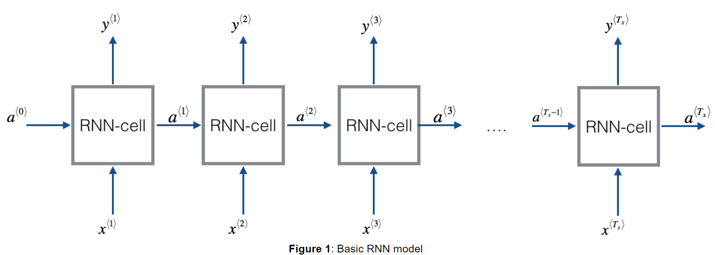
Later this week, you will generate music using an RNN. The basic RNN that you will implement has the structure below. In this example, Tx=Ty.
Here's how you can implement an RNN:
Steps:
- Implement the calculations needed for one time-step of the RNN.
- Implement a loop over Tx time-steps in order to process all the inputs, one at a time.
Let's go!
1.1 - RNN cell
A Recurrent neural network can be seen as the repetition of a single cell. You are first going to implement the computations for a single time-step. The following figure describes the operations for a single time-step of an RNN cell.
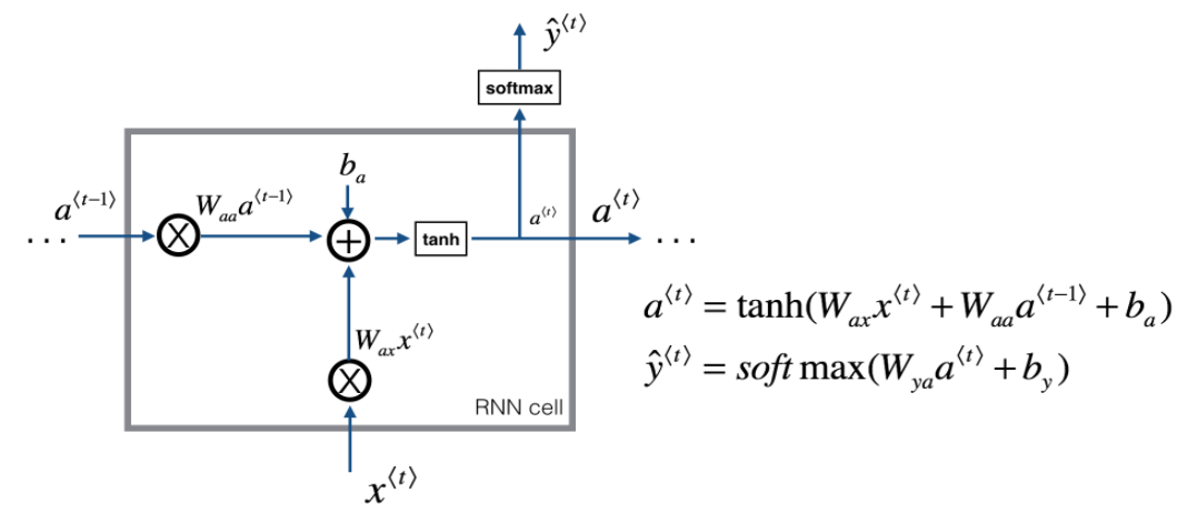
Figure 2: Basic RNN cell. Takes as input x⟨t⟩ (current input) and a⟨t−1⟩ (previous hidden state containing information from the past), and outputs a⟨t⟩ which is given to the next RNN cell and also used to predict y⟨t⟩
Exercise: Implement the RNN-cell described in Figure (2).
Instructions:
- Compute the hidden state with tanh activation: a⟨t⟩=tanh(Waaa⟨t−1⟩+Waxx⟨t⟩+ba).
- Using your new hidden state a⟨t⟩, compute the prediction ŷ ⟨t⟩=softmax(Wyaa⟨t⟩+by). We provided you a function:
softmax. - Store (a⟨t⟩,a⟨t−1⟩,x⟨t⟩,parameters) in cache
- Return a⟨t⟩ , y⟨t⟩ and cache
We will vectorize over m examples. Thus, x⟨t⟩ will have dimension (nx,m), and a⟨t⟩ will have dimension (na,m).
【code】
# GRADED FUNCTION: rnn_cell_forward

def rnn_cell_forward(xt, a_prev, parameters):
    """
    Implements a single forward step of the RNN-cell as described in Figure (2)

    Arguments:
    xt -- your input data at timestep "t", numpy array of shape (n_x, m).
    a_prev -- Hidden state at timestep "t-1", numpy array of shape (n_a, m)
    parameters -- python dictionary containing:
                        Wax -- Weight matrix multiplying the input, numpy array of shape (n_a, n_x)
                        Waa -- Weight matrix multiplying the hidden state, numpy array of shape (n_a, n_a)
                        Wya -- Weight matrix relating the hidden-state to the output, numpy array of shape (n_y, n_a)
                        ba --  Bias, numpy array of shape (n_a, 1)
                        by -- Bias relating the hidden-state to the output, numpy array of shape (n_y, 1)
    Returns:
    a_next -- next hidden state, of shape (n_a, m)
    yt_pred -- prediction at timestep "t", numpy array of shape (n_y, m)
    cache -- tuple of values needed for the backward pass, contains (a_next, a_prev, xt, parameters)
    """

    # Retrieve parameters from "parameters"
    Wax = parameters["Wax"]
    Waa = parameters["Waa"]
    Wya = parameters["Wya"]
    ba = parameters["ba"]
    by = parameters["by"]

    ### START CODE HERE ### (≈2 lines)
    # compute next activation state using the formula given above
    a_next = np.tanh(np.dot(Wax,xt) + np.dot(Waa,a_prev)+ ba )
    # compute output of the current cell using the formula given above
    yt_pred = softmax(np.dot(Wya,a_next)+ by)
    ### END CODE HERE ###

    # store values you need for backward propagation in cache
    cache = (a_next, a_prev, xt, parameters)

    return a_next, yt_pred, cache
np.random.seed(1)
xt = np.random.randn(3,10)
a_prev = np.random.randn(5,10)
Waa = np.random.randn(5,5)
Wax = np.random.randn(5,3)
Wya = np.random.randn(2,5)
ba = np.random.randn(5,1)
by = np.random.randn(2,1)
parameters = {"Waa": Waa, "Wax": Wax, "Wya": Wya, "ba": ba, "by": by}

a_next, yt_pred, cache = rnn_cell_forward(xt, a_prev, parameters)
print("a_next[4] = ", a_next[4])
print("a_next.shape = ", a_next.shape)
print("yt_pred[1] =", yt_pred[1])
print("yt_pred.shape = ", yt_pred.shape)
【result】
a_next[4] =  [ 0.59584544  0.18141802  0.61311866  0.99808218  0.85016201  0.99980978
 -0.18887155  0.99815551  0.6531151   0.82872037]
a_next.shape =  (5, 10)
yt_pred[1] = [ 0.9888161   0.01682021  0.21140899  0.36817467  0.98988387  0.88945212
  0.36920224  0.9966312   0.9982559   0.17746526]
yt_pred.shape =  (2, 10)
Expected Output:
| a_next[4]: | [ 0.59584544 0.18141802 0.61311866 0.99808218 0.85016201 0.99980978 -0.18887155 0.99815551 0.6531151 0.82872037] |
| a_next.shape: | (5, 10) |
| yt[1]: | [ 0.9888161 0.01682021 0.21140899 0.36817467 0.98988387 0.88945212 0.36920224 0.9966312 0.9982559 0.17746526] |
| yt.shape: | (2, 10) |
1.2 - RNN forward pass
You can see an RNN as the repetition of the cell you've just built. If your input sequence of data is carried over 10 time steps, then you will copy the RNN cell 10 times. Each cell takes as input the hidden state from the previous cell (a⟨t−1⟩) and the current time-step's input data (x⟨t⟩). It outputs a hidden state (a⟨t⟩) and a prediction (y⟨t⟩) for this time-step.
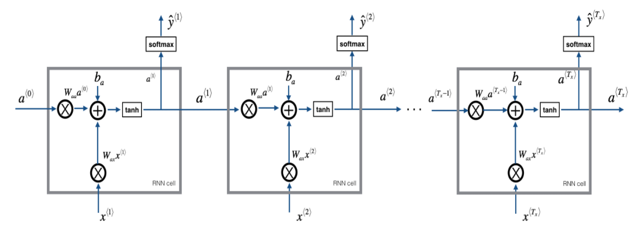
Exercise: Code the forward propagation of the RNN described in Figure (3).
Instructions:
- Create a vector of zeros (a) that will store all the hidden states computed by the RNN.
- Initialize the "next" hidden state as a0 (initial hidden state).
- Start looping over each time step, your incremental index is t :
- Update the "next" hidden state and the cache by running
rnn_cell_forward - Store the "next" hidden state in a (tth position)
- Store the prediction in y
- Add the cache to the list of caches
- Update the "next" hidden state and the cache by running
- Return a, y and caches
【中文翻译】
- 创建一个f zeros (a) 的向量, 它将存储由 RNN 计算的所有隐藏层状态。
- 将 "下一个" 隐藏层状态初始化为 a0 (初始隐藏层状态)。
- 在每次步骤开始循环时, 增量索引为 t:
- 通过运行 rnn_cell_forward 更新 "下一个" 隐藏层状态和缓存
- 在 a 中存储 "下一个" 隐藏层状态 (tth 位置)
- 将预测存储在 y 中
- 将缓存添加到缓存列表中
- 返回 a、y 和缓存
【code】
# GRADED FUNCTION: rnn_forward

def rnn_forward(x, a0, parameters):
    """
    Implement the forward propagation of the recurrent neural network described in Figure (3).

    Arguments:
    x -- Input data for every time-step, of shape (n_x, m, T_x).
    a0 -- Initial hidden state, of shape (n_a, m)
    parameters -- python dictionary containing:
                        Waa -- Weight matrix multiplying the hidden state, numpy array of shape (n_a, n_a)
                        Wax -- Weight matrix multiplying the input, numpy array of shape (n_a, n_x)
                        Wya -- Weight matrix relating the hidden-state to the output, numpy array of shape (n_y, n_a)
                        ba --  Bias numpy array of shape (n_a, 1)
                        by -- Bias relating the hidden-state to the output, numpy array of shape (n_y, 1)

    Returns:
    a -- Hidden states for every time-step, numpy array of shape (n_a, m, T_x)
    y_pred -- Predictions for every time-step, numpy array of shape (n_y, m, T_x)
    caches -- tuple of values needed for the backward pass, contains (list of caches, x)
    """

    # Initialize "caches" which will contain the list of all caches
    caches = []

    # Retrieve dimensions from shapes of x and parameters["Wya"]
    n_x, m, T_x = x.shape
    n_y, n_a = parameters["Wya"].shape

    ### START CODE HERE ###

    # initialize "a" and "y" with zeros (≈2 lines)
    a = np.zeros((n_a, m, T_x))
    y_pred = np.zeros((n_y, m, T_x))

    # Initialize a_next (≈1 line)
    a_next = a0

    # loop over all time-steps
    for t in range(T_x):
        # Update next hidden state, compute the prediction, get the cache (≈1 line)
        a_next, yt_pred, cache = rnn_cell_forward(x[:,:,t], a_next, parameters)
        # Save the value of the new "next" hidden state in a (≈1 line)
        a[:,:,t] = a_next
        # Save the value of the prediction in y (≈1 line)
        y_pred[:,:,t] = yt_pred
        # Append "cache" to "caches" (≈1 line)
        caches.append(cache)

    ### END CODE HERE ###

    # store values needed for backward propagation in cache
    caches = (caches, x)

    return a, y_pred, caches
np.random.seed(1)
x = np.random.randn(3,10,4)
a0 = np.random.randn(5,10)
Waa = np.random.randn(5,5)
Wax = np.random.randn(5,3)
Wya = np.random.randn(2,5)
ba = np.random.randn(5,1)
by = np.random.randn(2,1)
parameters = {"Waa": Waa, "Wax": Wax, "Wya": Wya, "ba": ba, "by": by}

a, y_pred, caches = rnn_forward(x, a0, parameters)
print("a[4][1] = ", a[4][1])
print("a.shape = ", a.shape)
print("y_pred[1][3] =", y_pred[1][3])
print("y_pred.shape = ", y_pred.shape)
print("caches[1][1][3] =", caches[1][1][3])
print("len(caches) = ", len(caches))
【result】
a[4][1] =  [-0.99999375  0.77911235 -0.99861469 -0.99833267]
a.shape =  (5, 10, 4)
y_pred[1][3] = [ 0.79560373  0.86224861  0.11118257  0.81515947]
y_pred.shape =  (2, 10, 4)
caches[1][1][3] = [-1.1425182  -0.34934272 -0.20889423  0.58662319]
len(caches) =  2
Expected Output:
| a[4][1]: | [-0.99999375 0.77911235 -0.99861469 -0.99833267] |
| a.shape: | (5, 10, 4) |
| y[1][3]: | [ 0.79560373 0.86224861 0.11118257 0.81515947] |
| y.shape: | (2, 10, 4) |
| cache[1][1][3]: | [-1.1425182 -0.34934272 -0.20889423 0.58662319] |
| len(cache): | 2 |
Congratulations! You've successfully built the forward propagation of a recurrent neural network from scratch. This will work well enough for some applications, but it suffers from vanishing gradient problems. So it works best when each output y⟨t⟩ can be estimated using mainly "local" context (meaning information from inputs x⟨t′⟩ where t′ is not too far from t).
In the next part, you will build a more complex LSTM model, which is better at addressing vanishing gradients. The LSTM will be better able to remember a piece of information and keep it saved for many timesteps.
2 - Long Short-Term Memory (LSTM) network
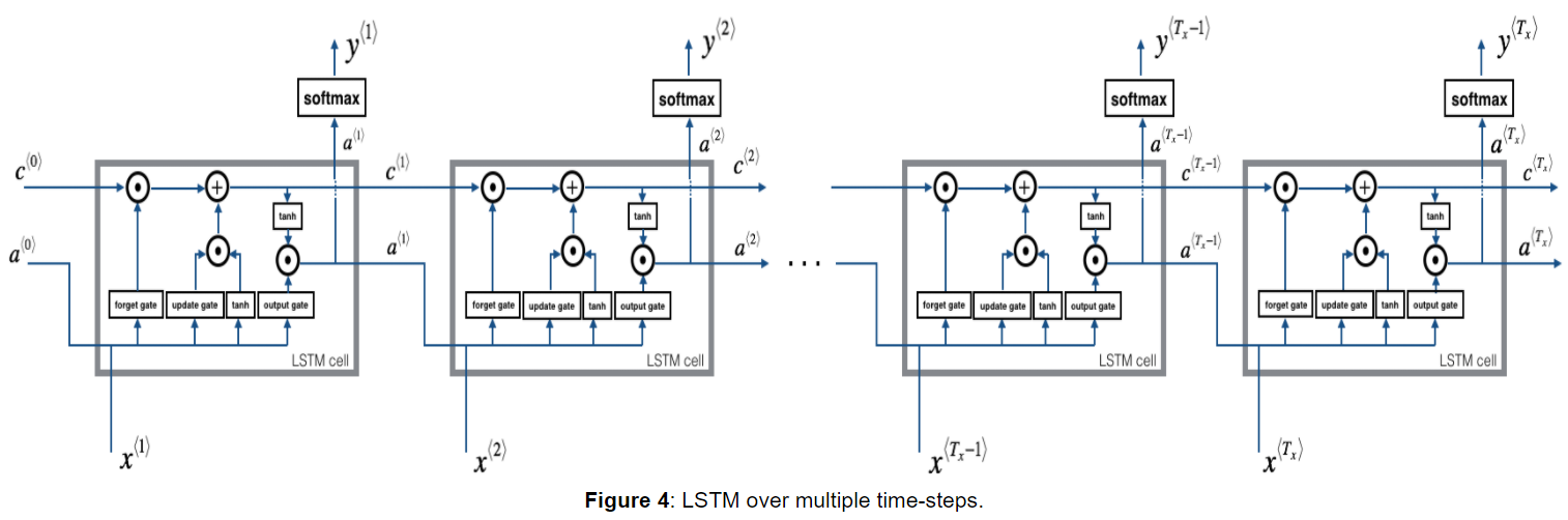
This following figure shows the operations of an LSTM-cell.
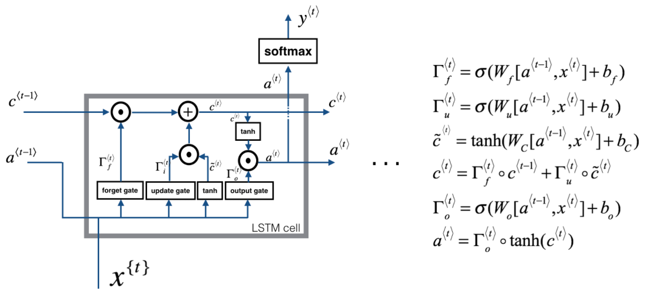
Figure 4: LSTM-cell. This tracks and updates a "cell state" or memory variable c⟨t⟩ at every time-step, which can be different from a⟨t⟩.
Similar to the RNN example above, you will start by implementing the LSTM cell for a single time-step. Then you can iteratively call it from inside a for-loop to have it process an input with Tx time-steps.
About the gates
- Forget gate
For the sake of this illustration, lets assume we are reading words in a piece of text, and want use an LSTM to keep track of grammatical structures, such as whether the subject is singular or plural. If the subject changes from a singular word to a plural word, we need to find a way to get rid of our previously stored memory value of the singular/plural state. In an LSTM, the forget gate lets us do this:
![]()
Here, Wf are weights that govern the forget gate's behavior. We concatenate [a⟨t−1⟩,x⟨t⟩] and multiply by Wf. The equation above results in a vector Γf⟨t⟩ with values between 0 and 1. This forget gate vector will be multiplied element-wise by the previous cell state c⟨t−1⟩. So if one of the values of Γf⟨t⟩ is 0 (or close to 0) then it means that the LSTM should remove that piece of information (e.g. the singular subject) in the corresponding component of c⟨t−1⟩. If one of the values is 1, then it will keep the information.
- Update gate
Once we forget that the subject being discussed is singular, we need to find a way to update it to reflect that the new subject is now plural. Here is the formulat for the update gate:
![]()
Similar to the forget gate, here Γu⟨t⟩ is again a vector of values between 0 and 1. This will be multiplied element-wise with c̃ ⟨t⟩, in order to compute c⟨t⟩.
- Updating the cell
To update the new subject we need to create a new vector of numbers that we can add to our previous cell state. The equation we use is:
Finally, the new cell state is:
![]()
- Output gate
To decide which outputs we will use, we will use the following two formulas:

Where in equation 5 you decide what to output using a sigmoid function and in equation 6 you multiply that by the tanh of the previous state.
【中文翻译】
![]()
在这里, Wf 是控制遗忘门行为的权重。我们连接 [a⟨t−1⟩,x⟨t⟩] , 乘以 Wf 。上面的等式导致向量Γf⟨t⟩值在0和1之间。这个忘记门向量将被乘以前细胞状态 c⟨t−1⟩。因此, 如果Γf⟨t⟩的值之一是 0 (或接近 0), 则表示 LSTM 应在 c⟨t−1⟩的相应组件中删除该信息 (如单数)。如果其中一个值为 1, 则它将保留该信息。
![]()
类似于遗忘门, 这里Γu⟨t⟩ 向量值在0和1之间。这将乘以c̃ ⟨t⟩, 以计算 c⟨t⟩。
![]()
最后, 新细胞状态为:
![]()
在等式5中, 你决定用一个 sigmoid函数输出什么, 在等式6中, 你乘以以前状态的 tanh。
2.1 - LSTM cell
Exercise: Implement the LSTM cell described in the Figure (3).
Instructions:
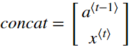
- Concatenate a⟨t−1⟩ and x⟨t⟩ in a single matrix:
- Compute all the formulas 1-6. You can use
sigmoid()(provided) andnp.tanh(). - Compute the prediction y⟨t⟩. You can use
softmax()(provided).
【code】
# GRADED FUNCTION: lstm_cell_forward

def lstm_cell_forward(xt, a_prev, c_prev, parameters):
    """
    Implement a single forward step of the LSTM-cell as described in Figure (4)

    Arguments:
    xt -- your input data at timestep "t", numpy array of shape (n_x, m).
    a_prev -- Hidden state at timestep "t-1", numpy array of shape (n_a, m)
    c_prev -- Memory state at timestep "t-1", numpy array of shape (n_a, m)
    parameters -- python dictionary containing:
                        Wf -- Weight matrix of the forget gate, numpy array of shape (n_a, n_a + n_x)
                        bf -- Bias of the forget gate, numpy array of shape (n_a, 1)
                        Wi -- Weight matrix of the update gate, numpy array of shape (n_a, n_a + n_x)
                        bi -- Bias of the update gate, numpy array of shape (n_a, 1)
                        Wc -- Weight matrix of the first "tanh", numpy array of shape (n_a, n_a + n_x)
                        bc --  Bias of the first "tanh", numpy array of shape (n_a, 1)
                        Wo -- Weight matrix of the output gate, numpy array of shape (n_a, n_a + n_x)
                        bo --  Bias of the output gate, numpy array of shape (n_a, 1)
                        Wy -- Weight matrix relating the hidden-state to the output, numpy array of shape (n_y, n_a)
                        by -- Bias relating the hidden-state to the output, numpy array of shape (n_y, 1)

    Returns:
    a_next -- next hidden state, of shape (n_a, m)
    c_next -- next memory state, of shape (n_a, m)
    yt_pred -- prediction at timestep "t", numpy array of shape (n_y, m)
    cache -- tuple of values needed for the backward pass, contains (a_next, c_next, a_prev, c_prev, xt, parameters)

    Note: ft/it/ot stand for the forget/update/output gates, cct stands for the candidate value (c tilde),
          c stands for the memory value
    """

    # Retrieve parameters from "parameters"
    Wf = parameters["Wf"]
    bf = parameters["bf"]
    Wi = parameters["Wi"]
    bi = parameters["bi"]
    Wc = parameters["Wc"]
    bc = parameters["bc"]
    Wo = parameters["Wo"]
    bo = parameters["bo"]
    Wy = parameters["Wy"]
    by = parameters["by"]

    # Retrieve dimensions from shapes of xt and Wy
    n_x, m = xt.shape
    n_y, n_a = Wy.shape

    ### START CODE HERE ###
    # Concatenate a_prev and xt (≈3 lines)

    # xt -- your input data at timestep "t", numpy array of shape (n_x, m).
    # a_prev -- Hidden state at timestep "t-1", numpy array of shape (n_a, m)

    concat = np.zeros([n_x+n_a,m])
    concat[: n_a, :] = a_prev
    concat[n_a :, :] = xt

    # Compute values for ft, it, cct, c_next, ot, a_next using the formulas given figure (4) (≈6 lines)
    ft = sigmoid(np.dot(Wf,concat)+bf)
    it = sigmoid(np.dot(Wi,concat)+bi)
    cct = np.tanh(np.dot(Wc,concat)+bc)
    c_next = ft*c_prev + it*cct
    ot = sigmoid(np.dot(Wo,concat)+bo)
    a_next =ot* np.tanh(c_next)

    # Compute prediction of the LSTM cell (≈1 line)
    yt_pred = softmax(a_next)
    ### END CODE HERE ###

    # store values needed for backward propagation in cache
    cache = (a_next, c_next, a_prev, c_prev, ft, it, cct, ot, xt, parameters)

    return a_next, c_next, yt_pred, cache
np.random.seed(1)
xt = np.random.randn(3,10)
a_prev = np.random.randn(5,10)
c_prev = np.random.randn(5,10)
Wf = np.random.randn(5, 5+3)
bf = np.random.randn(5,1)
Wi = np.random.randn(5, 5+3)
bi = np.random.randn(5,1)
Wo = np.random.randn(5, 5+3)
bo = np.random.randn(5,1)
Wc = np.random.randn(5, 5+3)
bc = np.random.randn(5,1)
Wy = np.random.randn(2,5)
by = np.random.randn(2,1)

parameters = {"Wf": Wf, "Wi": Wi, "Wo": Wo, "Wc": Wc, "Wy": Wy, "bf": bf, "bi": bi, "bo": bo, "bc": bc, "by": by}

a_next, c_next, yt, cache = lstm_cell_forward(xt, a_prev, c_prev, parameters)
print("a_next[4] = ", a_next[4])
print("a_next.shape = ", c_next.shape)
print("c_next[2] = ", c_next[2])
print("c_next.shape = ", c_next.shape)
print("yt[1] =", yt[1])
print("yt.shape = ", yt.shape)
print("cache[1][3] =", cache[1][3])
print("len(cache) = ", len(cache))
【result】
a_next[4] =  [-0.66408471  0.0036921   0.02088357  0.22834167 -0.85575339  0.00138482
  0.76566531  0.34631421 -0.00215674  0.43827275]
a_next.shape =  (5, 10)
c_next[2] =  [ 0.63267805  1.00570849  0.35504474  0.20690913 -1.64566718  0.11832942
  0.76449811 -0.0981561  -0.74348425 -0.26810932]
c_next.shape =  (5, 10)
yt[1] = [ 0.30831726  0.1609229   0.17145947  0.19722879  0.25181449  0.20285798
  0.08757126  0.19024486  0.14454214  0.17710263]
yt.shape =  (5, 10)
cache[1][3] = [-0.16263996  1.03729328  0.72938082 -0.54101719  0.02752074 -0.30821874
  0.07651101 -1.03752894  1.41219977 -0.37647422]
len(cache) =  10
Expected Output:
| a_next[4]: | [-0.66408471 0.0036921 0.02088357 0.22834167 -0.85575339 0.00138482 0.76566531 0.34631421 -0.00215674 0.43827275] |
| a_next.shape: | (5, 10) |
| c_next[2]: | [ 0.63267805 1.00570849 0.35504474 0.20690913 -1.64566718 0.11832942 0.76449811 -0.0981561 -0.74348425 -0.26810932] |
| c_next.shape: | (5, 10) |
| yt[1]: | [ 0.79913913 0.15986619 0.22412122 0.15606108 0.97057211 0.31146381 0.00943007 0.12666353 0.39380172 0.07828381] |
| yt.shape: | (2, 10) |
| cache[1][3]: | [-0.16263996 1.03729328 0.72938082 -0.54101719 0.02752074 -0.30821874 0.07651101 -1.03752894 1.41219977 -0.37647422] |
| len(cache): | 10 |
2.2 - Forward pass for LSTM
Now that you have implemented one step of an LSTM, you can now iterate this over this using a for-loop to process a sequence of Tx inputs.
Exercise: Implement lstm_forward() to run an LSTM over TxTx time-steps.
Note: c⟨0⟩ is initialized with zeros.
【code】
# GRADED FUNCTION: lstm_forward

def lstm_forward(x, a0, parameters):
    """
    Implement the forward propagation of the recurrent neural network using an LSTM-cell described in Figure (3).

    Arguments:
    x -- Input data for every time-step, of shape (n_x, m, T_x).
    a0 -- Initial hidden state, of shape (n_a, m)
    parameters -- python dictionary containing:
                        Wf -- Weight matrix of the forget gate, numpy array of shape (n_a, n_a + n_x)
                        bf -- Bias of the forget gate, numpy array of shape (n_a, 1)
                        Wi -- Weight matrix of the update gate, numpy array of shape (n_a, n_a + n_x)
                        bi -- Bias of the update gate, numpy array of shape (n_a, 1)
                        Wc -- Weight matrix of the first "tanh", numpy array of shape (n_a, n_a + n_x)
                        bc -- Bias of the first "tanh", numpy array of shape (n_a, 1)
                        Wo -- Weight matrix of the output gate, numpy array of shape (n_a, n_a + n_x)
                        bo -- Bias of the output gate, numpy array of shape (n_a, 1)
                        Wy -- Weight matrix relating the hidden-state to the output, numpy array of shape (n_y, n_a)
                        by -- Bias relating the hidden-state to the output, numpy array of shape (n_y, 1)

    Returns:
    a -- Hidden states for every time-step, numpy array of shape (n_a, m, T_x)
    y -- Predictions for every time-step, numpy array of shape (n_y, m, T_x)
    caches -- tuple of values needed for the backward pass, contains (list of all the caches, x)
    """

    # Initialize "caches", which will track the list of all the caches
    caches = []

    ### START CODE HERE ###
    # Retrieve dimensions from shapes of x and parameters['Wy'] (≈2 lines)
    n_x, m, T_x = x.shape
    n_y, n_a = parameters['Wy'].shape

    # initialize "a", "c" and "y" with zeros (≈3 lines)
    a = np.zeros([n_a, m, T_x])
    c = np.zeros([n_a, m, T_x])
    y = np.zeros([n_y, m, T_x])

    # Initialize a_next and c_next (≈2 lines)
    a_next = a0
    c_next = np.zeros([n_a, m])

    # loop over all time-steps
    for t in range(T_x):
        # Update next hidden state, next memory state, compute the prediction, get the cache (≈1 line)
        a_next, c_next, yt, cache = lstm_cell_forward(x[:,:,t], a_next, c_next, parameters)
        # Save the value of the new "next" hidden state in a (≈1 line)
        a[:,:,t] = a_next
        # Save the value of the prediction in y (≈1 line)
        y[:,:,t] = yt
        # Save the value of the next cell state (≈1 line)
        c[:,:,t]  = c_next
        # Append the cache into caches (≈1 line)
        caches.append(cache)

    ### END CODE HERE ###

    # store values needed for backward propagation in cache
    caches = (caches, x)

    return a, y, c, caches
np.random.seed(1)
x = np.random.randn(3,10,7)
a0 = np.random.randn(5,10)
Wf = np.random.randn(5, 5+3)
bf = np.random.randn(5,1)
Wi = np.random.randn(5, 5+3)
bi = np.random.randn(5,1)
Wo = np.random.randn(5, 5+3)
bo = np.random.randn(5,1)
Wc = np.random.randn(5, 5+3)
bc = np.random.randn(5,1)
Wy = np.random.randn(2,5)
by = np.random.randn(2,1)

parameters = {"Wf": Wf, "Wi": Wi, "Wo": Wo, "Wc": Wc, "Wy": Wy, "bf": bf, "bi": bi, "bo": bo, "bc": bc, "by": by}

a, y, c, caches = lstm_forward(x, a0, parameters)
print("a[4][3][6] = ", a[4][3][6])
print("a.shape = ", a.shape)
print("y[1][4][3] =", y[1][4][3])
print("y.shape = ", y.shape)
print("caches[1][1[1]] =", caches[1][1][1])
print("c[1][2][1]", c[1][2][1])
print("len(caches) = ", len(caches))
【result】
a[4][3][6] =  0.172117767533
a.shape =  (5, 10, 7)
y[1][4][3] = 0.95087346185
y.shape =  (2, 10, 7)
caches[1][1[1]] = [ 0.82797464  0.23009474  0.76201118 -0.22232814 -0.20075807  0.18656139
  0.41005165]
c[1][2][1] -0.855544916718
len(caches) =  2
Expected Output:
| a[4][3][6] = | 0.172117767533 |
| a.shape = | (5, 10, 7) |
| y[1][4][3] = | 0.95087346185 |
| y.shape = | (2, 10, 7) |
| caches[1][1][1] = | [ 0.82797464 0.23009474 0.76201118 -0.22232814 -0.20075807 0.18656139 0.41005165] |
| c[1][2][1] = | -0.855544916718 |
| len(caches) = | 2 |
Congratulations! You have now implemented the forward passes for the basic RNN and the LSTM. When using a deep learning framework, implementing the forward pass is sufficient to build systems that achieve great performance.
The rest of this notebook is optional, and will not be graded.
3.1 - Basic RNN backward pass
We will start by computing the backward pass for the basic RNN-cell.

Figure 5: RNN-cell's backward pass. Just like in a fully-connected neural network, the derivative of the cost function J backpropagates through the RNN by following the chain-rule from calculas. The chain-rule is also used to calculate ![]() to update the parameters
to update the parameters ![]()
Deriving the one step backward functions:
To compute the rnn_cell_backward you need to compute the following equations. It is a good exercise to derive them by hand.
The derivative of tanh is ![]() . You can find the complete proof here. Note that:
. You can find the complete proof here. Note that: ![]()
Similarly for ![]() , the derivative of tanh(u) is
, the derivative of tanh(u) is ![]() .
.
The final two equations also follow same rule and are derived using the tanhtanh derivative. Note that the arrangement is done in a way to get the same dimensions to match.
【code】
def rnn_cell_backward(da_next, cache):
    """
    Implements the backward pass for the RNN-cell (single time-step).

    Arguments:
    da_next -- Gradient of loss with respect to next hidden state
    cache -- python dictionary containing useful values (output of rnn_cell_forward())

    Returns:
    gradients -- python dictionary containing:
                        dx -- Gradients of input data, of shape (n_x, m)
                        da_prev -- Gradients of previous hidden state, of shape (n_a, m)
                        dWax -- Gradients of input-to-hidden weights, of shape (n_a, n_x)
                        dWaa -- Gradients of hidden-to-hidden weights, of shape (n_a, n_a)
                        dba -- Gradients of bias vector, of shape (n_a, 1)
    """

    # Retrieve values from cache
    (a_next, a_prev, xt, parameters) = cache

    # Retrieve values from parameters
    Wax = parameters["Wax"]
    Waa = parameters["Waa"]
    Wya = parameters["Wya"]
    ba = parameters["ba"]
    by = parameters["by"]

    ### START CODE HERE ###
    # compute the gradient of tanh with respect to a_next (≈1 line)  , dtanh 可以只看做一个中间结果的表示方式
    dtanh = (1- a_next**2) * da_next   #注意这里是 element_wise ,即 * da_next

    # compute the gradient of the loss with respect to Wax (≈2 lines)
    # 根据公式1、2, dxt =  da_next .(  Wax.T  . (1- tanh(a_next)**2) ) = da_next .(  Wax.T  . dtanh * (1/d_a_next) )= Wax.T  . dtanh
    # 根据公式1、3, dWax =  da_next .( (1- tanh(a_next)**2) . xt.T) = da_next .(  dtanh * (1/d_a_next) . xt.T )=  dtanh . xt.T
    # 上面的 . 表示 np.dot
    dxt = np.dot(Wax.T, dtanh)
    dWax =  np.dot(dtanh,xt.T)

    # compute the gradient with respect to Waa (≈2 lines)
    da_prev = np.dot(Waa.T, dtanh)
    dWaa = np.dot(dtanh,a_prev.T)

    # compute the gradient with respect to b (≈1 line)
    #   axis=0 列方向上操作 axis=1 行方向上操作  keepdims=True 矩阵的二维特性
    dba = np.sum(dtanh, axis=1, keepdims=True)

    ### END CODE HERE ###

    # Store the gradients in a python dictionary
    gradients = {"dxt": dxt, "da_prev": da_prev, "dWax": dWax, "dWaa": dWaa, "dba": dba}

    return gradients
np.random.seed(1)
xt = np.random.randn(3,10)
a_prev = np.random.randn(5,10)
Wax = np.random.randn(5,3)
Waa = np.random.randn(5,5)
Wya = np.random.randn(2,5)
b = np.random.randn(5,1)
by = np.random.randn(2,1)
parameters = {"Wax": Wax, "Waa": Waa, "Wya": Wya, "ba": ba, "by": by}

a_next, yt, cache = rnn_cell_forward(xt, a_prev, parameters)

da_next = np.random.randn(5,10)
gradients = rnn_cell_backward(da_next, cache)
print("gradients["dxt"][1][2] =", gradients["dxt"][1][2])
print("gradients["dxt"].shape =", gradients["dxt"].shape)
print("gradients["da_prev"][2][3] =", gradients["da_prev"][2][3])
print("gradients["da_prev"].shape =", gradients["da_prev"].shape)
print("gradients["dWax"][3][1] =", gradients["dWax"][3][1])
print("gradients["dWax"].shape =", gradients["dWax"].shape)
print("gradients["dWaa"][1][2] =", gradients["dWaa"][1][2])
print("gradients["dWaa"].shape =", gradients["dWaa"].shape)
print("gradients["dba"][4] =", gradients["dba"][4])
print("gradients["dba"].shape =", gradients["dba"].shape)
【result】
gradients["dxt"][1][2] = -0.460564103059
gradients["dxt"].shape = (3, 10)
gradients["da_prev"][2][3] = 0.0842968653807
gradients["da_prev"].shape = (5, 10)
gradients["dWax"][3][1] = 0.393081873922
gradients["dWax"].shape = (5, 3)
gradients["dWaa"][1][2] = -0.28483955787
gradients["dWaa"].shape = (5, 5)
gradients["dba"][4] = [ 0.80517166]
gradients["dba"].shape = (5, 1)
Expected Output:
| gradients["dxt"][1][2] = | -0.460564103059 |
| gradients["dxt"].shape = | (3, 10) |
| gradients["da_prev"][2][3] = | 0.0842968653807 |
| gradients["da_prev"].shape = | (5, 10) |
| gradients["dWax"][3][1] = | 0.393081873922 |
| gradients["dWax"].shape = | (5, 3) |
| gradients["dWaa"][1][2] = | -0.28483955787 |
| gradients["dWaa"].shape = | (5, 5) |
| gradients["dba"][4] = | [ 0.80517166] |
| gradients["dba"].shape = | (5, 1) |
Backward pass through the RNN
Computing the gradients of the cost with respect to a⟨t⟩ at every time-step t is useful because it is what helps the gradient backpropagate to the previous RNN-cell. To do so, you need to iterate through all the time steps starting at the end, and at each step, you increment the overall dba, dWaa, dWax and you store dx.
Instructions:
Implement the rnn_backward function. Initialize the return variables with zeros first and then loop through all the time steps while calling the rnn_cell_backward at each time timestep, update the other variables accordingly.
【中文翻译】
【code】
def rnn_backward(da, caches):
    """
    Implement the backward pass for a RNN over an entire sequence of input data.

    Arguments:
    da -- Upstream (上游)gradients of all hidden states, of shape (n_a, m, T_x)
    caches -- tuple containing information from the forward pass (rnn_forward)

    Returns:
    gradients -- python dictionary containing:
                        dx -- Gradient w.r.t. the input data, numpy-array of shape (n_x, m, T_x)
                        da0 -- Gradient w.r.t the initial hidden state, numpy-array of shape (n_a, m)
                        dWax -- Gradient w.r.t the input's weight matrix, numpy-array of shape (n_a, n_x)
                        dWaa -- Gradient w.r.t the hidden state's weight matrix, numpy-arrayof shape (n_a, n_a)
                        dba -- Gradient w.r.t the bias, of shape (n_a, 1)
    """

    ### START CODE HERE ###

    # Retrieve values from the first cache (t=1) of caches (≈2 lines)
    (caches, x) = caches
    (a1, a0, x1, parameters) = caches[0]  # t=1 时的值

    # Retrieve dimensions from da's and x1's shapes (≈2 lines)
    n_a, m, T_x = da.shape
    n_x, m = x1.shape

    # initialize the gradients with the right sizes (≈6 lines)
    dx = np.zeros((n_x, m, T_x))
    dWax = np.zeros(parameters["Wax"].shape)
    dWaa = np.zeros(parameters["Waa"].shape)
    dba = np.zeros(parameters["ba"].shape)
    da0 = np.zeros(a0.shape)
    da_prevt = np.zeros((n_a, m))

    # Loop through all the time steps
    for t in reversed(range(T_x)):
        # Compute gradients at time step t. Choose wisely the "da_next" and the "cache" to use in the backward propagation step. (≈1 line)
        gradients = rnn_cell_backward(da[:,:,t] + da_prevt, caches[t]) # da[:,:,t] + da_prevt ,每一个时间步后更新梯度
        # Retrieve derivatives from gradients (≈ 1 line)
        dxt, da_prevt, dWaxt, dWaat, dbat = gradients["dxt"], gradients["da_prev"], gradients["dWax"], gradients["dWaa"], gradients["dba"]
        # Increment global derivatives w.r.t parameters by adding their derivative at time-step t (≈4 lines)
        dx[:, :, t] = dxt
        dWax += dWaxt
        dWaa += dWaat
        dba += dbat

    # Set da0 to the gradient of a which has been backpropagated through all time-steps (≈1 line)
    da0 = da_prevt
    ### END CODE HERE ###

    # Store the gradients in a python dictionary
    gradients = {"dx": dx, "da0": da0, "dWax": dWax, "dWaa": dWaa,"dba": dba}

    return gradients
np.random.seed(1)
x = np.random.randn(3,10,4)
a0 = np.random.randn(5,10)
Wax = np.random.randn(5,3)
Waa = np.random.randn(5,5)
Wya = np.random.randn(2,5)
ba = np.random.randn(5,1)
by = np.random.randn(2,1)
parameters = {"Wax": Wax, "Waa": Waa, "Wya": Wya, "ba": ba, "by": by}
a, y, caches = rnn_forward(x, a0, parameters)
da = np.random.randn(5, 10, 4)
gradients = rnn_backward(da, caches)

print("gradients["dx"][1][2] =", gradients["dx"][1][2])
print("gradients["dx"].shape =", gradients["dx"].shape)
print("gradients["da0"][2][3] =", gradients["da0"][2][3])
print("gradients["da0"].shape =", gradients["da0"].shape)
print("gradients["dWax"][3][1] =", gradients["dWax"][3][1])
print("gradients["dWax"].shape =", gradients["dWax"].shape)
print("gradients["dWaa"][1][2] =", gradients["dWaa"][1][2])
print("gradients["dWaa"].shape =", gradients["dWaa"].shape)
print("gradients["dba"][4] =", gradients["dba"][4])
print("gradients["dba"].shape =", gradients["dba"].shape)
【result】
gradients["dx"][1][2] = [-2.07101689 -0.59255627  0.02466855  0.01483317]
gradients["dx"].shape = (3, 10, 4)
gradients["da0"][2][3] = -0.314942375127
gradients["da0"].shape = (5, 10)
gradients["dWax"][3][1] = 11.2641044965
gradients["dWax"].shape = (5, 3)
gradients["dWaa"][1][2] = 2.30333312658
gradients["dWaa"].shape = (5, 5)
gradients["dba"][4] = [-0.74747722]
gradients["dba"].shape = (5, 1)
【Expected Output】
gradients["dx"][1][2] =	[-2.07101689 -0.59255627 0.02466855 0.01483317]
gradients["dx"].shape =	(3, 10, 4)
gradients["da0"][2][3] =	-0.314942375127
gradients["da0"].shape =	(5, 10)
gradients["dWax"][3][1] =	11.2641044965
gradients["dWax"].shape =	(5, 3)
gradients["dWaa"][1][2] =	2.30333312658
gradients["dWaa"].shape =	(5, 5)
gradients["dba"][4] =	[-0.74747722]
gradients["dba"].shape =	(5, 1)
3.2 - LSTM backward pass
3.2.1 One Step backward
The LSTM backward pass is slighltly more complicated than the forward one. We have provided you with all the equations for the LSTM backward pass below. (If you enjoy calculus exercises feel free to try deriving these from scratch yourself.)
3.2.2 gate derivatives
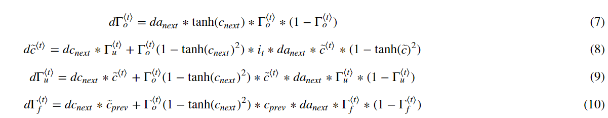
注:
(1)公式(8)中的it代表什么?it 代表 Γu⟨t⟩ ?
(2)公式10中c̃prev 代表 cprev ?
(3)上面的*代表element-wise ,即元素乘积
(4)公式好像有错误
3.2.3 parameter derivatives
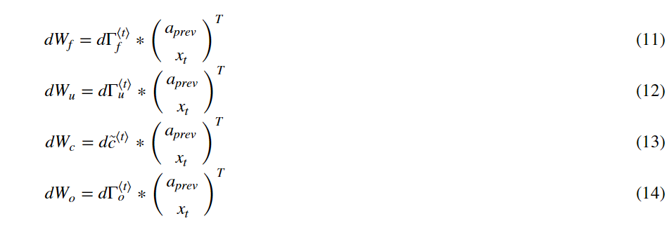
注: 上面的公式用的是*,即element-wise,这里的公式应该点乘,即np.dot()
To calculate dbf,dbu,dbc,dbo you just need to sum across the horizontal (axis= 1) axis on dΓf⟨t⟩,dΓu⟨t⟩,dc̃ ⟨t⟩,dΓo⟨t⟩ respectively. Note that you should have the keep_dims = True option.
Finally, you will compute the derivative with respect to the previous hidden state, previous memory state, and input.
![]()
Here, the weights for equations 13 are the first n_a, (i.e. Wf=Wf[:na,:] etc...)

where the weights for equation 15 are from n_a to the end, (i.e. Wf=Wf[na:,:] etc...)
注:
(1)上面的公式(15)、(17)用的是*,即element-wise,这里的公式应该点乘,即np.dot()
(2)上面的公式(16)用的是*,即element-wise,不用np.dot()
Exercise: Implement lstm_cell_backward by implementing equations 7−17 below. Good luck! :)
【code】
def lstm_cell_backward(da_next, dc_next, cache):
    """
    Implement the backward pass for the LSTM-cell (single time-step).

    Arguments:
    da_next -- Gradients of next hidden state, of shape (n_a, m)
    dc_next -- Gradients of next cell state, of shape (n_a, m)
    cache -- cache storing information from the forward pass

    Returns:
    gradients -- python dictionary containing:
                        dxt -- Gradient of input data at time-step t, of shape (n_x, m)
                        da_prev -- Gradient w.r.t. the previous hidden state, numpy array of shape (n_a, m)
                        dc_prev -- Gradient w.r.t. the previous memory state, of shape (n_a, m, T_x)
                        dWf -- Gradient w.r.t. the weight matrix of the forget gate, numpy array of shape (n_a, n_a + n_x)
                        dWi -- Gradient w.r.t. the weight matrix of the update gate, numpy array of shape (n_a, n_a + n_x)
                        dWc -- Gradient w.r.t. the weight matrix of the memory gate, numpy array of shape (n_a, n_a + n_x)
                        dWo -- Gradient w.r.t. the weight matrix of the output gate, numpy array of shape (n_a, n_a + n_x)
                        dbf -- Gradient w.r.t. biases of the forget gate, of shape (n_a, 1)
                        dbi -- Gradient w.r.t. biases of the update gate, of shape (n_a, 1)
                        dbc -- Gradient w.r.t. biases of the memory gate, of shape (n_a, 1)
                        dbo -- Gradient w.r.t. biases of the output gate, of shape (n_a, 1)
    """

    # Retrieve information from "cache"
    (a_next, c_next, a_prev, c_prev, ft, it, cct, ot, xt, parameters) = cache

    ### START CODE HERE ###
    # Retrieve dimensions from xt's and a_next's shape (≈2 lines)
    n_x, m = xt.shape
    n_a, m = a_next.shape

    # Compute gates related derivatives, you can find their values can be found by looking carefully at equations (7) to (10) (≈4 lines)
    dot = da_next * np.tanh(c_next) * ot * (1 - ot)
    dcct = (dc_next * it + ot * (1 - np.square(np.tanh(c_next))) * it * da_next) * (1 - np.square(cct))
    dit = (dc_next * cct + ot * (1 - np.square(np.tanh(c_next))) * cct * da_next) * it * (1 - it)
    dft = (dc_next * c_prev + ot *(1 - np.square(np.tanh(c_next))) * c_prev * da_next) * ft * (1 - ft)

    # 连接矩阵
    concat = np.concatenate((a_prev, xt), axis=0)

    # Compute parameters related derivatives. Use equations (11)-(14) (≈8 lines)
    dWf = np.dot(dft, concat.T)
    dWi = np.dot(dit, concat.T)
    dWc = np.dot(dcct, concat.T)
    dWo = np.dot(dot, concat.T)
    dbf = np.sum(dft, axis=1 ,keepdims = True)
    dbi = np.sum(dit, axis=1, keepdims = True)
    dbc = np.sum(dcct, axis=1,  keepdims = True)
    dbo = np.sum(dot, axis=1, keepdims = True)

    # Compute derivatives w.r.t previous hidden state, previous memory state and input. Use equations (15)-(17). (≈3 lines)
    # parameters['Wf'][:, :n_a].T 每一行的 第 0 到 n_a-1 列的数据取出来
    # parameters['Wf'][:, n_a:].T 每一行的 第 n_a 到最后列的数据取出来
    da_prev = np.dot(parameters['Wf'][:, :n_a].T, dft) + np.dot(parameters['Wi'][:, :n_a].T, dit) + np.dot(parameters['Wc'][:, :n_a].T, dcct) + np.dot(parameters['Wo'][:, :n_a].T, dot)
    dc_prev = dc_next * ft + ot * (1 - np.square(np.tanh(c_next))) * ft * da_next
    dxt = np.dot(parameters['Wf'][:, n_a:].T, dft) + np.dot(parameters['Wi'][:, n_a:].T, dit) + np.dot(parameters['Wc'][:, n_a:].T, dcct) + np.dot(parameters['Wo'][:, n_a:].T, dot)
    ### END CODE HERE ###

    # Save gradients in dictionary
    gradients = {"dxt": dxt, "da_prev": da_prev, "dc_prev": dc_prev, "dWf": dWf,"dbf": dbf, "dWi": dWi,"dbi": dbi,
                "dWc": dWc,"dbc": dbc, "dWo": dWo,"dbo": dbo}

    return gradients
np.random.seed(1)
xt = np.random.randn(3,10)
a_prev = np.random.randn(5,10)
c_prev = np.random.randn(5,10)
Wf = np.random.randn(5, 5+3)
bf = np.random.randn(5,1)
Wi = np.random.randn(5, 5+3)
bi = np.random.randn(5,1)
Wo = np.random.randn(5, 5+3)
bo = np.random.randn(5,1)
Wc = np.random.randn(5, 5+3)
bc = np.random.randn(5,1)
Wy = np.random.randn(2,5)
by = np.random.randn(2,1)

parameters = {"Wf": Wf, "Wi": Wi, "Wo": Wo, "Wc": Wc, "Wy": Wy, "bf": bf, "bi": bi, "bo": bo, "bc": bc, "by": by}

a_next, c_next, yt, cache = lstm_cell_forward(xt, a_prev, c_prev, parameters)

da_next = np.random.randn(5,10)
dc_next = np.random.randn(5,10)
gradients = lstm_cell_backward(da_next, dc_next, cache)
print("gradients["dxt"][1][2] =", gradients["dxt"][1][2])
print("gradients["dxt"].shape =", gradients["dxt"].shape)
print("gradients["da_prev"][2][3] =", gradients["da_prev"][2][3])
print("gradients["da_prev"].shape =", gradients["da_prev"].shape)
print("gradients["dc_prev"][2][3] =", gradients["dc_prev"][2][3])
print("gradients["dc_prev"].shape =", gradients["dc_prev"].shape)
print("gradients["dWf"][3][1] =", gradients["dWf"][3][1])
print("gradients["dWf"].shape =", gradients["dWf"].shape)
print("gradients["dWi"][1][2] =", gradients["dWi"][1][2])
print("gradients["dWi"].shape =", gradients["dWi"].shape)
print("gradients["dWc"][3][1] =", gradients["dWc"][3][1])
print("gradients["dWc"].shape =", gradients["dWc"].shape)
print("gradients["dWo"][1][2] =", gradients["dWo"][1][2])
print("gradients["dWo"].shape =", gradients["dWo"].shape)
print("gradients["dbf"][4] =", gradients["dbf"][4])
print("gradients["dbf"].shape =", gradients["dbf"].shape)
print("gradients["dbi"][4] =", gradients["dbi"][4])
print("gradients["dbi"].shape =", gradients["dbi"].shape)
print("gradients["dbc"][4] =", gradients["dbc"][4])
print("gradients["dbc"].shape =", gradients["dbc"].shape)
print("gradients["dbo"][4] =", gradients["dbo"][4])
print("gradients["dbo"].shape =", gradients["dbo"].shape)
【result】
gradients["dxt"][1][2] = 3.23055911511
gradients["dxt"].shape = (3, 10)
gradients["da_prev"][2][3] = -0.0639621419711
gradients["da_prev"].shape = (5, 10)
gradients["dc_prev"][2][3] = 0.797522038797
gradients["dc_prev"].shape = (5, 10)
gradients["dWf"][3][1] = -0.147954838164
gradients["dWf"].shape = (5, 8)
gradients["dWi"][1][2] = 1.05749805523
gradients["dWi"].shape = (5, 8)
gradients["dWc"][3][1] = 2.30456216369
gradients["dWc"].shape = (5, 8)
gradients["dWo"][1][2] = 0.331311595289
gradients["dWo"].shape = (5, 8)
gradients["dbf"][4] = [ 0.18864637]
gradients["dbf"].shape = (5, 1)
gradients["dbi"][4] = [-0.40142491]
gradients["dbi"].shape = (5, 1)
gradients["dbc"][4] = [ 0.25587763]
gradients["dbc"].shape = (5, 1)
gradients["dbo"][4] = [ 0.13893342]
gradients["dbo"].shape = (5, 1)
【Expected Output】
gradients["dxt"][1][2] =	3.23055911511
gradients["dxt"].shape =	(3, 10)
gradients["da_prev"][2][3] =	-0.0639621419711
gradients["da_prev"].shape =	(5, 10)
gradients["dc_prev"][2][3] =	0.797522038797
gradients["dc_prev"].shape =	(5, 10)
gradients["dWf"][3][1] =	-0.147954838164
gradients["dWf"].shape =	(5, 8)
gradients["dWi"][1][2] =	1.05749805523
gradients["dWi"].shape =	(5, 8)
gradients["dWc"][3][1] =	2.30456216369
gradients["dWc"].shape =	(5, 8)
gradients["dWo"][1][2] =	0.331311595289
gradients["dWo"].shape =	(5, 8)
gradients["dbf"][4] =	[ 0.18864637]
gradients["dbf"].shape =	(5, 1)
gradients["dbi"][4] =	[-0.40142491]
gradients["dbi"].shape =	(5, 1)
gradients["dbc"][4] =	[ 0.25587763]
gradients["dbc"].shape =	(5, 1)
gradients["dbo"][4] =	[ 0.13893342]
gradients["dbo"].shape =	(5, 1)
3.3 Backward pass through the LSTM RNN
This part is very similar to the rnn_backward function you implemented above. You will first create variables of the same dimension as your return variables. You will then iterate over all the time steps starting from the end and call the one step function you implemented for LSTM at each iteration. You will then update the parameters by summing them individually. Finally return a dictionary with the new gradients.
Instructions: Implement the lstm_backward function. Create a for loop starting from Tx and going backward. For each step call lstm_cell_backward and update the your old gradients by adding the new gradients to them. Note that dxt is not updated but is stored.
【中文翻译】
【code】
def lstm_backward(da, caches):

    """
    Implement the backward pass for the RNN with LSTM-cell (over a whole sequence).

    Arguments:
    da -- Gradients w.r.t the hidden states, numpy-array of shape (n_a, m, T_x)
    dc -- Gradients w.r.t the memory states, numpy-array of shape (n_a, m, T_x)
    caches -- cache storing information from the forward pass (lstm_forward)

    Returns:
    gradients -- python dictionary containing:
                        dx -- Gradient of inputs, of shape (n_x, m, T_x)
                        da0 -- Gradient w.r.t. the previous hidden state, numpy array of shape (n_a, m)
                        dWf -- Gradient w.r.t. the weight matrix of the forget gate, numpy array of shape (n_a, n_a + n_x)
                        dWi -- Gradient w.r.t. the weight matrix of the update gate, numpy array of shape (n_a, n_a + n_x)
                        dWc -- Gradient w.r.t. the weight matrix of the memory gate, numpy array of shape (n_a, n_a + n_x)
                        dWo -- Gradient w.r.t. the weight matrix of the save gate, numpy array of shape (n_a, n_a + n_x)
                        dbf -- Gradient w.r.t. biases of the forget gate, of shape (n_a, 1)
                        dbi -- Gradient w.r.t. biases of the update gate, of shape (n_a, 1)
                        dbc -- Gradient w.r.t. biases of the memory gate, of shape (n_a, 1)
                        dbo -- Gradient w.r.t. biases of the save gate, of shape (n_a, 1)
    """

    # Retrieve values from the first cache (t=1) of caches.
    (caches, x) = caches
    (a1, c1, a0, c0, f1, i1, cc1, o1, x1, parameters) = caches[0]

    ### START CODE HERE ###
    # Retrieve dimensions from da's and x1's shapes (≈2 lines)
    n_a, m, T_x = da.shape
    n_x, m = x1.shape

    # initialize the gradients with the right sizes (≈12 lines)
    dx = np.zeros((n_x, m, T_x))
    da0 = np.zeros((n_a, m))
    da_prevt = np.zeros((n_a, m))
    dc_prevt = np.zeros((n_a, m))
    dWf = np.zeros((n_a, n_a + n_x))
    dWi = np.zeros((n_a, n_a + n_x))
    dWc = np.zeros((n_a, n_a + n_x))
    dWo = np.zeros((n_a, n_a + n_x))
    dbf = np.zeros((n_a, 1))
    dbi = np.zeros((n_a, 1))
    dbc = np.zeros((n_a, 1))
    dbo = np.zeros((n_a, 1))


    # loop back over the whole sequence
    for t in reversed(range(T_x)):
        # Compute all gradients using lstm_cell_backward
        gradients = lstm_cell_backward(da[:, :, t], dc_prevt, caches[t])
        # Store or add the gradient to the parameters' previous step's gradient
        dx[:,:,t] = gradients["dxt"]
        dWf += gradients["dWf"]
        dWi += gradients["dWi"]
        dWc += gradients["dWc"]
        dWo += gradients["dWo"]
        dbf += gradients["dbf"]
        dbi += gradients["dbi"]     #输出值与期望值不一致
        dbc += gradients["dbc"]     #输出值与期望值不一致
        dbo += gradients["dbo"]     #输出值与期望值不一致
    # Set the first activation's gradient to the backpropagated gradient da_prev.
    da0 = gradients["da_prev"]

    ### END CODE HERE ###

    # Store the gradients in a python dictionary
    gradients = {"dx": dx, "da0": da0, "dWf": dWf,"dbf": dbf, "dWi": dWi,"dbi": dbi,
                "dWc": dWc,"dbc": dbc, "dWo": dWo,"dbo": dbo}

    return gradients
np.random.seed(1)
x = np.random.randn(3,10,7)
a0 = np.random.randn(5,10)
Wf = np.random.randn(5, 5+3)
bf = np.random.randn(5,1)
Wi = np.random.randn(5, 5+3)
bi = np.random.randn(5,1)
Wo = np.random.randn(5, 5+3)
bo = np.random.randn(5,1)
Wc = np.random.randn(5, 5+3)
bc = np.random.randn(5,1)

parameters = {"Wf": Wf, "Wi": Wi, "Wo": Wo, "Wc": Wc, "Wy": Wy, "bf": bf, "bi": bi, "bo": bo, "bc": bc, "by": by}

a, y, c, caches = lstm_forward(x, a0, parameters)

da = np.random.randn(5, 10, 4)
gradients = lstm_backward(da, caches)

print("gradients["dx"][1][2] =", gradients["dx"][1][2])
print("gradients["dx"].shape =", gradients["dx"].shape)
print("gradients["da0"][2][3] =", gradients["da0"][2][3])
print("gradients["da0"].shape =", gradients["da0"].shape)
print("gradients["dWf"][3][1] =", gradients["dWf"][3][1])
print("gradients["dWf"].shape =", gradients["dWf"].shape)
print("gradients["dWi"][1][2] =", gradients["dWi"][1][2])
print("gradients["dWi"].shape =", gradients["dWi"].shape)
print("gradients["dWc"][3][1] =", gradients["dWc"][3][1])
print("gradients["dWc"].shape =", gradients["dWc"].shape)
print("gradients["dWo"][1][2] =", gradients["dWo"][1][2])
print("gradients["dWo"].shape =", gradients["dWo"].shape)
print("gradients["dbf"][4] =", gradients["dbf"][4])
print("gradients["dbf"].shape =", gradients["dbf"].shape)
print("gradients["dbi"][4] =", gradients["dbi"][4])
print("gradients["dbi"].shape =", gradients["dbi"].shape)
print("gradients["dbc"][4] =", gradients["dbc"][4])
print("gradients["dbc"].shape =", gradients["dbc"].shape)
print("gradients["dbo"][4] =", gradients["dbo"][4])
print("gradients["dbo"].shape =", gradients["dbo"].shape)
【result】
gradients["dx"][1][2] = [-0.00173313  0.08287442 -0.30545663 -0.43281115]
gradients["dx"].shape = (3, 10, 4)
gradients["da0"][2][3] = -0.095911501954
gradients["da0"].shape = (5, 10)
gradients["dWf"][3][1] = -0.0698198561274
gradients["dWf"].shape = (5, 8)
gradients["dWi"][1][2] = 0.102371820249
gradients["dWi"].shape = (5, 8)
gradients["dWc"][3][1] = -0.0624983794927
gradients["dWc"].shape = (5, 8)
gradients["dWo"][1][2] = 0.0484389131444
gradients["dWo"].shape = (5, 8)
gradients["dbf"][4] = [-0.0565788]
gradients["dbf"].shape = (5, 1)
gradients["dbi"][4] = [-0.01339511]
gradients["dbi"].shape = (5, 1)
gradients["dbc"][4] = [-0.21783941]
gradients["dbc"].shape = (5, 1)
gradients["dbo"][4] = [ 0.22190701]
gradients["dbo"].shape = (5, 1)
【Expected Output】
gradients["dx"][1][2] =	[-0.00173313 0.08287442 -0.30545663 -0.43281115]
gradients["dx"].shape =	(3, 10, 4)
gradients["da0"][2][3] =	-0.095911501954
gradients["da0"].shape =	(5, 10)
gradients["dWf"][3][1] =	-0.0698198561274
gradients["dWf"].shape =	(5, 8)
gradients["dWi"][1][2] =	0.102371820249
gradients["dWi"].shape =	(5, 8)
gradients["dWc"][3][1] =	-0.0624983794927
gradients["dWc"].shape =	(5, 8)
gradients["dWo"][1][2] =	0.0484389131444
gradients["dWo"].shape =	(5, 8)
gradients["dbf"][4] =	[-0.0565788]
gradients["dbf"].shape =	(5, 1)
gradients["dbi"][4] =	[-0.06997391]
gradients["dbi"].shape =	(5, 1)
gradients["dbc"][4] =	[-0.27441821]
gradients["dbc"].shape =	(5, 1)
gradients["dbo"][4] =	[ 0.16532821]
gradients["dbo"].shape =	(5, 1)
Congratulations !
Congratulations on completing this assignment. You now understand how recurrent neural networks work!
Lets go on to the next exercise, where you'll use an RNN to build a character-level language model.
--------------------------------------------------------
参考链接:
1、http://blog.csdn.net/JUNJUN_ZHAO/article/details/79400107