一个隐含层的平面数据分类
2020-07-21
欢迎来到第三周的编程作业。现在是构建第一个神经网络的时候了,它有一个隐藏层。您将看到此模型与使用逻辑回归实现的模型之间的巨大差异。
您将学习如何:
•实现一个只有一个隐藏层的2分类神经网络
•使用具有非线性激活函数的单元,如tanh
•计算交叉熵损失
•实现向前和向后传播
本文作业是在jupyter notebook上一步一步做的,带有一些过程中查找的资料等(出处已标明)并翻译成了中文,如有错误,欢迎指正!
1 - Packages(包)
让我们首先导入在此任务中需要的所有包。
•numpy是使用Python进行科学计算的基本包。
•sklearn为数据挖掘和数据分析提供了简单而高效的工具。
matplotlib是Python中用于绘制图形的库。
testcase提供了一些测试示例来评估函数的正确性
planar_utils提供了在这个赋值中使用的各种有用的函数
# Package imports
import numpy as np
import matplotlib.pyplot as plt
from testCases import *
import sklearn
import sklearn.datasets
import sklearn.linear_model
from planar_utils import plot_decision_boundary, sigmoid, load_planar_dataset, load_extra_datasets

%matplotlib inline #这行代码是由于在jupyter上运行才要的
#可以将matplotlib的图表直接嵌入到Notebook之中,或者使用指定的界面库显示图表,它有一个参数指定matplotlib图表的显示方式。inline表示将图表嵌入到Notebook中
#有了%matplotlib inline 就可以省掉plt.show()了
np.random.seed(1) # set a seed so that the results are consistent
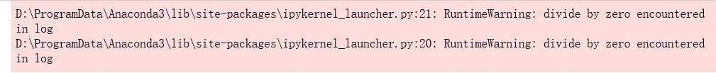
python中我们常会用到numpy.random.seed()函数。
其基本用法或作用网上很多人都写过:
seed( ) 用于指定随机数生成时所用算法开始的整数值,如果使用相同的seed( )值,则每次生成的随即数都相同
2 - Dataset(数据集)
First, let's get the dataset you will work on. The following code will load a "flower" 2-class dataset into variables X and Y.
首先,让我们获得要处理的数据集。下面的代码将把一个“flower”2分类 数据集加载到变量X和Y中。
X, Y = load_planar_dataset()
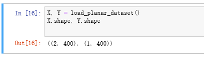
可以看到向量X是2X400就是2行400列,而Y是1X400就是1行400列
使用matplotlib可视化数据集。数据看起来像一朵“花”,有一些红色(标签y=0)和一些蓝色(y=1)点。您的目标是构建一个模型来匹配这些数据。
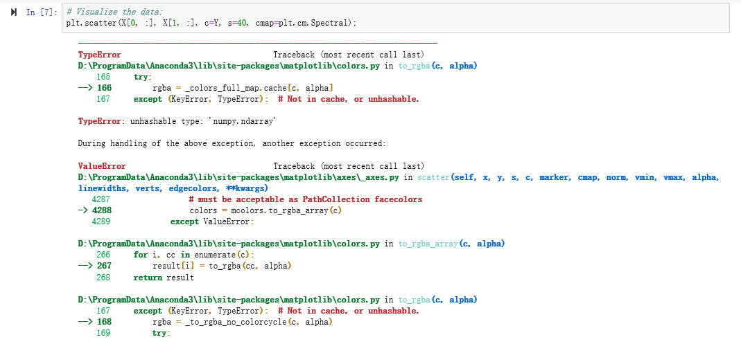
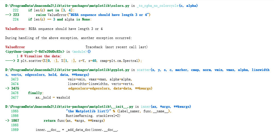
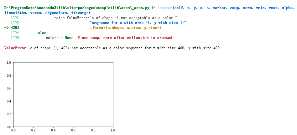
# Visualize the data:
plt.scatter(X[0, :], X[1, :], c=Y, s=40, cmap=plt.cm.Spectral);
(由于使用Jupyter Notebook在这周作业出现问题,运行不通过)问题如下:
参考了来自Miss思的吴恩达深度学习——第一课第三周课后编程作业Debug经历,链接:https://blog.csdn.net/weixin_43978140/article/details/85012675
以下转自:https://blog.csdn.net/weixin_43978140/article/details/85012675
1、数据可视化
#plt.scatter(X[0, :], X[1, :], c=Y, s=40, cmap=plt.cm.Spectral)
plt.scatter(X[0,:],X[1,:],c=np.squeeze(Y),*s=40,cmap=plt.cm.Spectral)
这里进行数据可视化的时候,纯用c=Y会出错,出错原因及解决方法如下:
在机器学习和深度学习中,通常算法的结果是可以表示向量的数组(即包含两对或以上的方括号形式[[]]),如果直接利用这个数组进行画图可能显示界面为空(见后面的示例)。
我们可以利用squeeze()函数将表示向量的数组转换为秩为1的数组,这样利用matplotlib库函数画图时,就可以正常的显示结果了。
2、关于plot_decision_boundar函数
这里主要也是要注意里面的参数,Y的部分要变成np.squeeze(Y)
更改代码后:
# Visualize the data:
plt.scatter(X[0, :], X[1, :], c= np.squeeze(Y), s=40, cmap=plt.cm.Spectral);

(plt.scatter( ) 函数的使用方法), 来自:春江明月


matplotlib.pyplot.scatter(x, y, s=None, c=None, marker=None, cmap=None, norm=None, vmin=None, vmax=None, alpha=None, linewidths=None, verts=None, edgecolors=None, *, data=None, **kwargs)
参数的解释:

x,y:表示的是大小为(n,)的数组,也就是我们即将绘制散点图的数据点

s:是一个实数或者是一个数组大小为(n,),这个是一个可选的参数。

c:表示的是颜色,也是一个可选项。默认是蓝色'b',表示的是标记的颜色,或者可以是一个表示颜色的字符,或者是一个长度为n的表示颜色的序列等等,感觉还没用到过现在不解释了。但是c不可以是一个单独的RGB数字,也不可以是一个RGBA的序列。可以是他们的2维数组(只有一行)。

marker:表示的是标记的样式,默认的是'o'。

cmap:Colormap实体或者是一个colormap的名字,cmap仅仅当c是一个浮点数数组的时候才使用。如果没有申明就是image.cmap

norm:Normalize实体来将数据亮度转化到0-1之间,也是只有c是一个浮点数的数组的时候才使用。如果没有申明,就是默认为colors.Normalize。

vmin,vmax:实数,当norm存在的时候忽略。用来进行亮度数据的归一化。

alpha:实数,0-1之间。

linewidths:也就是标记点的长度。
python中 x[:,0]和x[:,1] 理解和实例解析,来自jobschu
这里X[0, :]为第一行的所有数,X[1, :]为第二行的所有数
你有:
一个包含你的特征(x1, x2)的数字数组(矩阵)X
一个包含标签(红色:0,蓝色:1)的数字数组(向量)Y。
首先让我们更好地了解我们的数据是什么样的。
练习:你有多少训练例子?另外,变量X和Y的形状是什么?
提示:如何得到一个numpy数组的形状?(帮助)
### START CODE HERE ### (≈ 3 lines of code)
shape_X = X.shape
shape_Y = Y.shape
m = shape_X[1]  # training set size
### END CODE HERE ###

print ('The shape of X is: ' + str(shape_X))
print ('The shape of Y is: ' + str(shape_Y))
print ('I have m = %d training examples!' % (m))
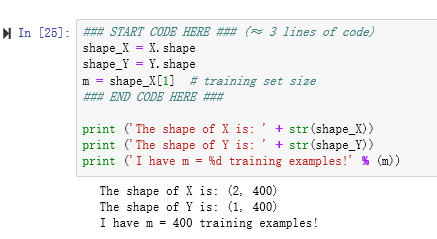
这里m = shape_X[1] # training set size,1是代表横轴的方向,所以有400个训练样本
3 - Simple Logistic Regression(简单逻辑回归)
在建立一个完整的神经网络之前,让我们先看看逻辑回归在这个问题上的表现。您可以使用sklearn的内置函数来实现这一点。运行下面的代码来训练数据集上的逻辑回归分类器。
# Train the logistic regression classifier
clf = sklearn.linear_model.LogisticRegressionCV();
clf.fit(X.T, Y.T);
注意上面的代码的Y也是需要转换为秩为1的数字:
# Train the logistic regression classifier
clf = sklearn.linear_model.LogisticRegressionCV();
clf.fit(X.T, np.squeeze(Y).T);
看到还有一种:
# Train the logistic regression classifier
clf = sklearn.linear_model.LogisticRegressionCV();
clf.fit(X.T, Y.T.ravel());#将多维数组降位一维
numpy中的ravel()、flatten()、squeeze()的用法与区别 - 草稿,来自:爱学习的大丁
fit()训练。调用fit(x,y)的方法来训练模型,其中x为数据的属性,y为所属类型。来自:静悟生慧,LogisticRegression回归算法 Sklearn 参数详解
sklearn逻辑回归(Logistic Regression,LR)类库使用小结,来自 :sun_shengyun,原文出处:http://www.cnblogs.com/pinard/p/6035872.html,在原文的基础上做了一些修订
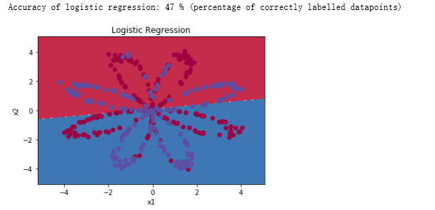
现在可以绘制这些模型的决策边界。运行下面的代码。
# Plot the decision boundary for logistic regression 绘制逻辑回归的决策边界
plot_decision_boundary(lambda x: clf.predict(x), X, Y)
plt.title("Logistic Regression")

# Print accuracy 打印精度
LR_predictions = clf.predict(X.T) #得到预测值Y_hat,标签
print ('Accuracy of logistic regression: %d ' % float((np.dot(Y,LR_predictions) + np.dot(1-Y,1-LR_predictions))/float(Y.size)*100) +
       '% ' + "(percentage of correctly labelled datapoints)")
绘制逻辑回归的决策边界是不是就是红蓝的分解线呢?
float((np.dot(Y,LR_predictions) + np.dot(1-Y,1-LR_predictions))/float(Y.size)*100)
到这里代码有些看不懂,plot_decision_boundary,这是一个函数吗?从最上面导入的情况来看是从属于planar_utils这个文件的,这个文件写了4个函数,如下
 1 import matplotlib.pyplot as plt
 2 import numpy as np
 3 import sklearn
 4 import sklearn.datasets
 5 import sklearn.linear_model
 6
 7 def plot_decision_boundary(model, X, y):
 8     # Set min and max values and give it some padding
 9     x_min, x_max = X[0, :].min() - 1, X[0, :].max() + 1
10     y_min, y_max = X[1, :].min() - 1, X[1, :].max() + 1
11     h = 0.01
12     # Generate a grid of points with distance h between them
13     xx, yy = np.meshgrid(np.arange(x_min, x_max, h), np.arange(y_min, y_max, h))
14     # Predict the function value for the whole grid
15     Z = model(np.c_[xx.ravel(), yy.ravel()])
16     Z = Z.reshape(xx.shape)
17     # Plot the contour and training examples
18     plt.contourf(xx, yy, Z, cmap=plt.cm.Spectral)
19     plt.ylabel('x2')
20     plt.xlabel('x1')
21     plt.scatter(X[0, :], X[1, :], c=np.squeeze(y), cmap=plt.cm.Spectral)
22
23
24 def sigmoid(x):
25     """
26     Compute the sigmoid of x
27
28     Arguments:
29     x -- A scalar or numpy array of any size.
30
31     Return:
32     s -- sigmoid(x)
33     """
34     s = 1/(1+np.exp(-x))
35     return s
36
37 def load_planar_dataset():
38     np.random.seed(1)
39     m = 400 # number of examples
40     N = int(m/2) # number of points per class
41     D = 2 # dimensionality
42     X = np.zeros((m,D)) # data matrix where each row is a single example
43     Y = np.zeros((m,1), dtype='uint8') # labels vector (0 for red, 1 for blue)
44     a = 4 # maximum ray of the flower
45
46     for j in range(2):
47         ix = range(N*j,N*(j+1))
48         t = np.linspace(j*3.12,(j+1)*3.12,N) + np.random.randn(N)*0.2 # theta
49         r = a*np.sin(4*t) + np.random.randn(N)*0.2 # radius
50         X[ix] = np.c_[r*np.sin(t), r*np.cos(t)]
51         Y[ix] = j
52
53     X = X.T
54     Y = Y.T
55
56     return X, Y
57
58 def load_extra_datasets():
59     N = 200
60     noisy_circles = sklearn.datasets.make_circles(n_samples=N, factor=.5, noise=.3)
61     noisy_moons = sklearn.datasets.make_moons(n_samples=N, noise=.2)
62     blobs = sklearn.datasets.make_blobs(n_samples=N, random_state=5, n_features=2, centers=6)
63     gaussian_quantiles = sklearn.datasets.make_gaussian_quantiles(mean=None, cov=0.5, n_samples=N, n_features=2, n_classes=2, shuffle=True, random_state=None)
64     no_structure = np.random.rand(N, 2), np.random.rand(N, 2)
65
66     return noisy_circles, noisy_moons, blobs, gaussian_quantiles, no_structure
解释:首先Y.size是400,因为Y是1X400的一个行向量,
可以看到逻辑回归分类准确率很低,无法正确分类。
解释:数据集不是线性可分的,所以logistic回归的效果不是很好。希望神经网络能做得更好。我们现在就来试试!
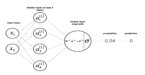
4 - Neural Network model
逻辑回归在“花数据集”上效果不佳。你要训练一个只有一个隐含层的神经网络。
Here is our model:
数学上的:
对于一个样本的xi:
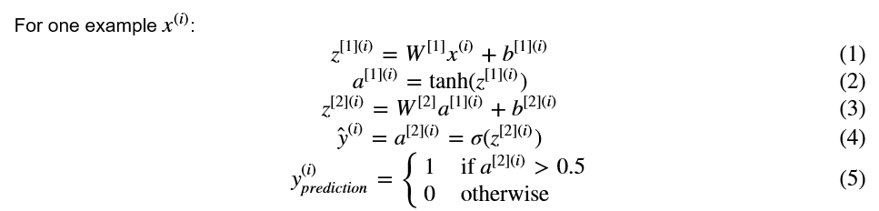
根据对所有例子的预测,您还可以计算代价J如下:

提醒:构建神经网络的一般方法是:
1. 定义神经网络结构(输入单元,隐藏单元,等等)。
2. 初始化模型的参数
3.循环:
实现正向传播
计算损失
实现反向传播,以获得梯度
更新参数(梯度下降)
您经常构建辅助函数来计算步骤1-3,然后将它们合并到一个称为nn_model()的函数中。一旦构建了nn_model()并学习了正确的参数,就可以对新数据进行预测。
4.1 -定义神经网络结构
练习:定义三个变量:
- n_x:输入层的大小
- n_h:隐藏层的大小(设置为4)
- n_y:输出层的大小
提示:使用X和Y的形状来查找n_x和n_y。同时,将隐藏层的大小硬编码为4。
# GRADED FUNCTION: layer_sizes

def layer_sizes(X, Y):
    """
    Arguments:
    X -- input dataset of shape (input size, number of examples)
    Y -- labels of shape (output size, number of examples)

    Returns:
    n_x -- the size of the input layer
    n_h -- the size of the hidden layer
    n_y -- the size of the output layer
    """
    ### START CODE HERE ### (≈ 3 lines of code)
    n_x = X.shape[0] # size of input layer X是2X400,2是不是就是2个特征,红和蓝其中为1
    n_h = 4
    n_y = Y.shape[0] # size of output layer Y是1X400
    ### END CODE HERE ###
    return (n_x, n_h, n_y)
X_assess, Y_assess = layer_sizes_test_case()
(n_x, n_h, n_y) = layer_sizes(X_assess, Y_assess)
print("The size of the input layer is: n_x = " + str(n_x))
print("The size of the hidden layer is: n_h = " + str(n_h))
print("The size of the output layer is: n_y = " + str(n_y))
结果:
The size of the input layer is: n_x = 5
The size of the hidden layer is: n_h = 4
The size of the output layer is: n_y = 2
预期输出(这不是您将用于网络的大小,它们只是用于评估您刚刚编写的函数)。
4.2 - Initialize the model's parameters(初始化模型的参数)
练习:实现函数initialize_parameters()。
说明:
•确保参数大小正确。如有需要,请参考上面的神经网络图。
•您将用随机值初始化权重矩阵。
◾使用:np.random.randn (a, b) * 0.01随机初始化一个矩阵的形状(a, b)。
•将偏差向量初始化为零。
◾使用:np.zeros ((a, b))来初始化一个矩阵的形状与0 (a, b)。
# GRADED FUNCTION: initialize_parameters

def initialize_parameters(n_x, n_h, n_y):
    """
    Argument:
    n_x -- size of the input layer
    n_h -- size of the hidden layer
    n_y -- size of the output layer

    Returns:
    params -- python dictionary containing your parameters:
                    W1 -- weight matrix of shape (n_h, n_x)
                    b1 -- bias vector of shape (n_h, 1)
                    W2 -- weight matrix of shape (n_y, n_h)
                    b2 -- bias vector of shape (n_y, 1)
    """

    np.random.seed(2) # we set up a seed so that your output matches ours although the initialization is random.

    ### START CODE HERE ### (≈ 4 lines of code)
    W1 = np.random.randn(n_h, n_x) * 0.01
    b1 = np.zeros((n_h, 1))
    W2 = np.random.randn(n_y, n_h) * 0.01
    b2 = np.zeros((n_y, 1))
    ### END CODE HERE ###

    assert (W1.shape == (n_h, n_x))
    assert (b1.shape == (n_h, 1))
    assert (W2.shape == (n_y, n_h))
    assert (b2.shape == (n_y, 1))

    parameters = {"W1": W1,
                  "b1": b1,
                  "W2": W2,
                  "b2": b2}

    return parameters
n_x, n_h, n_y = initialize_parameters_test_case()

parameters = initialize_parameters(n_x, n_h, n_y)
print("W1 = " + str(parameters["W1"]))
print("b1 = " + str(parameters["b1"]))
print("W2 = " + str(parameters["W2"]))
print("b2 = " + str(parameters["b2"]))
4.3 - The Loop(循环)
Question: Implement forward_propagation().(问题:实现forward_propagation ()。)
说明:
•看看上面的分类器的数学表示。
•可以使用函数sigmoid()。它是内置(导入)在笔记本电脑。
•可以使用函数np.tanh()。它是numpy库的一部分。
•你必须执行的步骤是:
1、通过使用parameters[".."],从字典"parameters" (是initialize_parameters()的输出)中检索每个参数。
2、实现向前传播。计算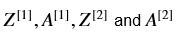 (你对训练集中所有例子的所有预测的向量)。
•反向传播所需的值存储在“缓存”中。缓存将作为反向传播函数的输入。
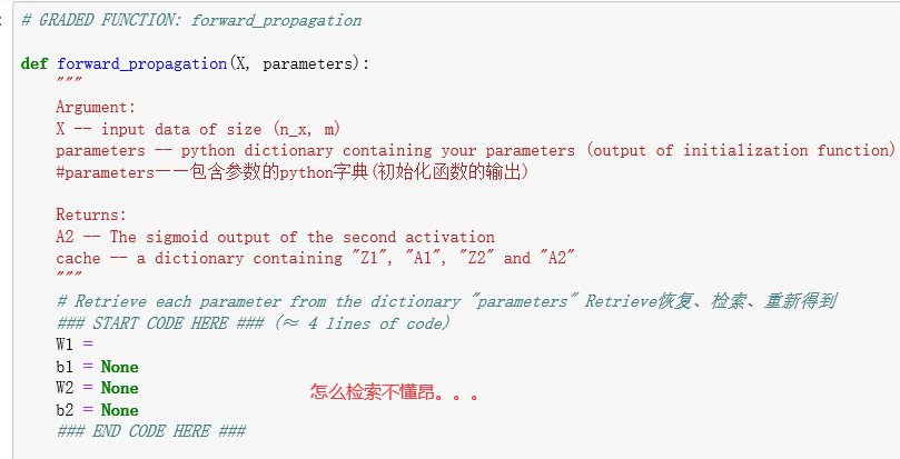
向前传播:
# GRADED FUNCTION: forward_propagation 先前传播

def forward_propagation(X, parameters):
    """
    Argument:
    X -- input data of size (n_x, m)
    parameters -- python dictionary containing your parameters (output of initialization function)
    #parameters——包含参数的python字典(初始化函数的输出)

    Returns:
    A2 -- The sigmoid output of the second activation
    cache -- a dictionary containing "Z1", "A1", "Z2" and "A2"
    """
    # Retrieve each parameter from the dictionary "parameters" Retrieve恢复、检索、重新得到
    ### START CODE HERE ### (≈ 4 lines of code)
    W1 = parameters["W1"]
    b1 = parameters["b1"]
    W2 = parameters["W2"]
    b2 = parameters["b2"]
    ### END CODE HERE ###

    # Implement Forward Propagation to calculate A2 (probabilities)
    ### START CODE HERE ### (≈ 4 lines of code)
    Z1 = np.dot(W1, X) + b1
    A1 = np.tanh(Z1)
    Z2 = np.dot(W2, A1) + b2
    A2 = sigmoid(Z2)
    ### END CODE HERE ###

    assert(A2.shape == (1, X.shape[1]))

    cache = {"Z1": Z1,
             "A1": A1,
             "Z2": Z2,
             "A2": A2}

    return A2, cache
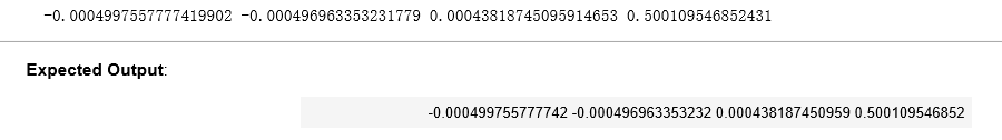
X_assess, parameters = forward_propagation_test_case()

A2, cache = forward_propagation(X_assess, parameters)

# Note: we use the mean here just to make sure that your output matches ours. 注意:我们在这里使用平均值只是为了确保您的输出与我们的匹配。
print(np.mean(cache['Z1']) ,np.mean(cache['A1']),np.mean(cache['Z2']),np.mean(cache['A2']))
现在你已经算出了A【2】(在Python中是变量“A2”),其中对于每个样本都包含了一个a【2】(i),你可以计算成本函数如下:
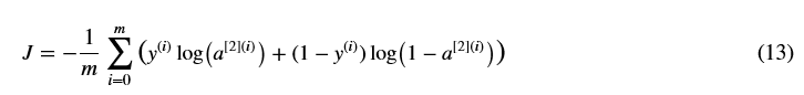
练习:实现compute_cost()来计算代价J的值
说明:•有很多方法可以实现交叉熵损失。为了帮助你,我们告诉你我们将如何实施:
logprobs = np.multiply(np.log(A2),Y)
cost = - np.sum(logprobs) # no need to use a for loop!
(you can use either np.multiply() and then np.sum() or directly np.dot()).
# GRADED FUNCTION: compute_cost

def compute_cost(A2, Y, parameters):
    """
    Computes the cross-entropy cost given in equation (13)

    Arguments:
    A2 -- The sigmoid output of the second activation, of shape (1, number of examples)
    Y -- "true" labels vector of shape (1, number of examples)
    parameters -- python dictionary containing your parameters W1, b1, W2 and b2

    Returns:
    cost -- cross-entropy cost given equation (13)
    """

    m = Y.shape[1] # number of example

    # Compute the cross-entropy cost
    ### START CODE HERE ### (≈ 2 lines of code)
    logprobs = np.multiply(np.log(A2), Y)
    cost = - np.sum(logprobs  + (1-Y) * np.log(1 - A2)) / m
    ### END CODE HERE ###

    cost = np.squeeze(cost)     # makes sure cost is the dimension we expect.
                                # E.g., turns [[17]] into 17
    assert(isinstance(cost, float))

    return cost
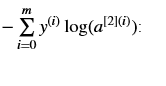
A2, Y_assess, parameters = compute_cost_test_case()

print("cost = " + str(compute_cost(A2, Y_assess, parameters)))
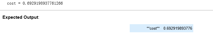
使用前向传播期间计算的缓存,现在可以实现后向传播。
问题:实现函数backward_propagation()。
说明:反向传播通常是深度学习中最难的部分。为了帮助你们,这里有一张关于反向传播的幻灯片。您需要使用这张幻灯片右边的六个方程,因为您正在构建一个向量化的实现。
提示:

# GRADED FUNCTION: backward_propagation

def backward_propagation(parameters, cache, X, Y):
    """
    Implement the backward propagation using the instructions above.

    Arguments:
    parameters -- python dictionary containing our parameters
    cache -- a dictionary containing "Z1", "A1", "Z2" and "A2".
    X -- input data of shape (2, number of examples)
    Y -- "true" labels vector of shape (1, number of examples)

    Returns:
    grads -- python dictionary containing your gradients with respect to different parameters
    """
    m = X.shape[1]

    # First, retrieve W1 and W2 from the dictionary "parameters".
    ### START CODE HERE ### (≈ 2 lines of code)
    W1 = parameters["W1"]
    W2 = parameters["W2"]
    ### END CODE HERE ###

    # Retrieve also A1 and A2 from dictionary "cache".
    ### START CODE HERE ### (≈ 2 lines of code)
    A1 = cache["A1"]
    A2 = cache["A2"]
    ### END CODE HERE ###

    # Backward propagation: calculate dW1, db1, dW2, db2.
    ### START CODE HERE ### (≈ 6 lines of code, corresponding to 6 equations on slide above)
    dZ2 = A2 - Y
    dW2 = np.dot(dZ2, A1.T) / m
    db2 = np.sum(dZ2, axis = 1, keepdims = True) / m
    dZ1 = np.multiply(W2.T * dZ2, (1 - np.power(A1, 2)))
    dW1 = np.dot(dZ1, X.T) / m
    db1 = np.sum(dZ1, axis = 1, keepdims = True) / m
    ### END CODE HERE ###

    grads = {"dW1": dW1,
             "db1": db1,
             "dW2": dW2,
             "db2": db2}

    return grads
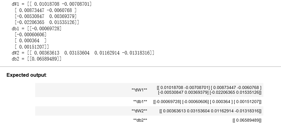
parameters, cache, X_assess, Y_assess = backward_propagation_test_case()

grads = backward_propagation(parameters, cache, X_assess, Y_assess)
print ("dW1 = "+ str(grads["dW1"]))
print ("db1 = "+ str(grads["db1"]))
print ("dW2 = "+ str(grads["dW2"]))
print ("db2 = "+ str(grads["db2"]))
问题:实现更新规则。用梯度下降法。为了更新(W1、b1、W2、b2),必须使用(dW1、db1、dW2、db2)。
一般梯度下降规则: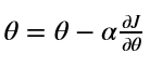 式中,α为学习率,θ代表参数。
说明:学习率好的梯度下降算法(收敛)和坏的学习率(发散)。图片由亚当·哈雷提供。

# GRADED FUNCTION: update_parameters

def update_parameters(parameters, grads, learning_rate = 1.2):
    """
    Updates parameters using the gradient descent update rule given above

    Arguments:
    parameters -- python dictionary containing your parameters
    grads -- python dictionary containing your gradients

    Returns:
    parameters -- python dictionary containing your updated parameters
    """
    # Retrieve each parameter from the dictionary "parameters"
    ### START CODE HERE ### (≈ 4 lines of code)
    W1 = parameters["W1"]
    b1 = parameters["b1"]
    W2 = parameters["W2"]
    b2 = parameters["b2"]
    ### END CODE HERE ###

    # Retrieve each gradient from the dictionary "grads"
    ### START CODE HERE ### (≈ 4 lines of code)
    dW1 = grads["dW1"]
    db1 = grads["db1"]
    dW2 = grads["dW2"]
    db2 = grads["db2"]
    ## END CODE HERE ###

    # Update rule for each parameter
    ### START CODE HERE ### (≈ 4 lines of code)
    W1 -= learning_rate * dW1
    b1 -= learning_rate * db1
    W2 -= learning_rate * dW2
    b2 -= learning_rate * db2
    ### END CODE HERE ###

    parameters = {"W1": W1,
                  "b1": b1,
                  "W2": W2,
                  "b2": b2}

    return parameters
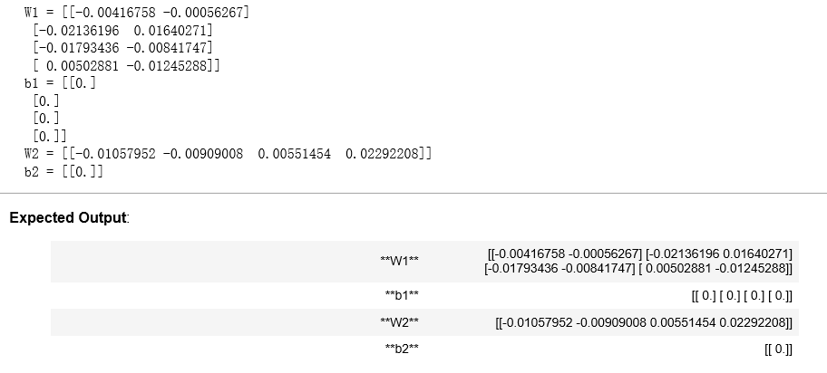
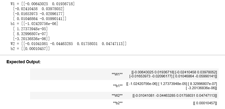
parameters, grads = update_parameters_test_case()
parameters = update_parameters(parameters, grads)

print("W1 = " + str(parameters["W1"]))
print("b1 = " + str(parameters["b1"]))
print("W2 = " + str(parameters["W2"]))
print("b2 = " + str(parameters["b2"]))
结果:
4.4 - Integrate parts 4.1, 4.2 and 4.3 in nn_model() (4.4 -整合nn_model()中的4.1、4.2、4.3部分)
问题:在nn_model()构建你的神经网络模型。
说明:神经网络模型必须按照正确的顺序使用前面的函数。
 1 # GRADED FUNCTION: nn_model
 2
 3 def nn_model(X, Y, n_h, num_iterations = 10000, print_cost=False):
 4     """
 5     Arguments:
 6     X -- dataset of shape (2, number of examples)
 7     Y -- labels of shape (1, number of examples)
 8     n_h -- size of the hidden layer
 9     num_iterations -- Number of iterations in gradient descent loop
10     print_cost -- if True, print the cost every 1000 iterations
11
12     Returns:
13     parameters -- parameters learnt by the model. They can then be used to predict.
14     """
15
16     np.random.seed(3)
17     n_x = layer_sizes(X, Y)[0]
18     n_y = layer_sizes(X, Y)[2]
19
20     # Initialize parameters, then retrieve W1, b1, W2, b2. Inputs: "n_x, n_h, n_y". Outputs = "W1, b1, W2, b2, parameters".
21     ### START CODE HERE ### (≈ 5 lines of code)
22     parameters = initialize_parameters(n_x, n_h, n_y)
23     W1 = parameters["W1"]
24     b1 = parameters["b1"]
25     W2 = parameters["W2"]
26     b2 = parameters["b2"]
27     ### END CODE HERE ###
28
29     # Loop (gradient descent)
30
31     for i in range(0, num_iterations):
32
33         ### START CODE HERE ### (≈ 4 lines of code)
34         # Forward propagation. Inputs: "X, parameters". Outputs: "A2, cache".
35         A2, cache = forward_propagation(X, parameters)
36
37         # Cost function. Inputs: "A2, Y, parameters". Outputs: "cost".
38         cost = compute_cost(A2, Y, parameters)
39
40         # Backpropagation. Inputs: "parameters, cache, X, Y". Outputs: "grads".
41         grads = backward_propagation(parameters, cache, X, Y)
42
43         # Gradient descent parameter update. Inputs: "parameters, grads". Outputs: "parameters".
44         parameters = update_parameters(parameters, grads)
45
46         ### END CODE HERE ###
47
48         # Print the cost every 1000 iterations
49         if print_cost and i % 1000 == 0:
50             print ("Cost after iteration %i: %f" %(i, cost))
51
52
53
54     return parameters
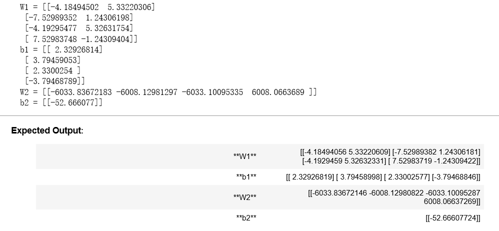
X_assess, Y_assess = nn_model_test_case()
parameters = nn_model(X_assess, Y_assess, 4, num_iterations=10000, print_cost=False)
print("W1 = " + str(parameters["W1"]))
print("b1 = " + str(parameters["b1"]))
print("W2 = " + str(parameters["W2"]))
print("b2 = " + str(parameters["b2"]))
结果:
4.5 Predictions
问题:通过构建predict()来使用您的模型进行预测。使用正向传播来预测结果。
提示: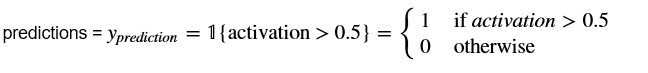
例如,如果您想根据阈值将矩阵X的项设置为0和1,您可以这样做:X_new = (X >阈值)
# GRADED FUNCTION: predict

def predict(parameters, X):
    """
    Using the learned parameters, predicts a class for each example in X

    Arguments:
    parameters -- python dictionary containing your parameters
    X -- input data of size (n_x, m)

    Returns
    predictions -- vector of predictions of our model (red: 0 / blue: 1)
    """

    # Computes probabilities using forward propagation, and classifies to 0/1 using 0.5 as the threshold.
    ### START CODE HERE ### (≈ 2 lines of code)
    A2, cache = forward_propagation(X, parameters) #A2就是y hat
    predictions = np.round(A2)
    #round() 方法返回浮点数x的四舍五入值。
    ### END CODE HERE ###

    return predictions
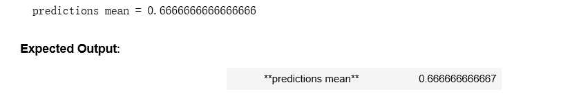
parameters, X_assess = predict_test_case()

predictions = predict(parameters, X_assess)
print("predictions mean = " + str(np.mean(predictions)))
结果:
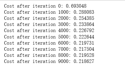
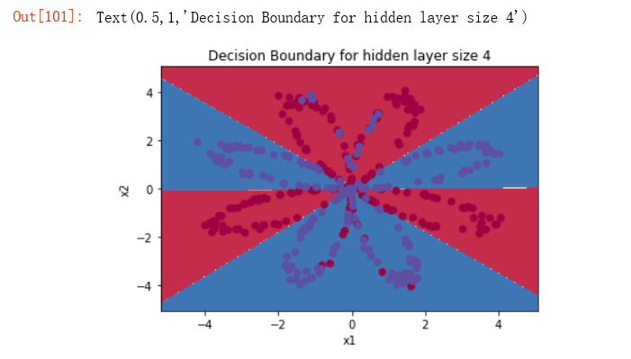
现在是时候运行模型,看看它在平面数据集上的表现如何。运行下面的代码,用一个隐藏层来测试您的模型,nh隐藏的单位。
# Build a model with a n_h-dimensional hidden layer
parameters = nn_model(X, Y, n_h = 4, num_iterations = 10000, print_cost=True) #这里n_h = 4 是隐藏层的神经元个数哦

# Plot the decision boundary
plot_decision_boundary(lambda x: predict(parameters, x.T), X, Y)
plt.title("Decision Boundary for hidden layer size " + str(4))
结果:
# Print accuracy
predictions = predict(parameters, X)
print ('Accuracy: %d' % float((np.dot(Y,predictions.T) + np.dot(1-Y,1-predictions.T))/float(Y.size)*100) + '%')
结果:
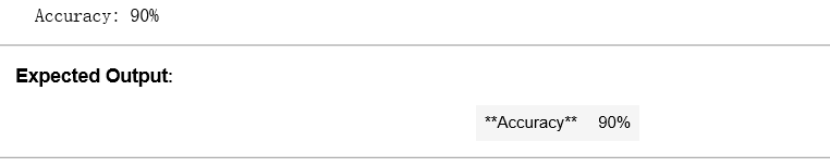
与逻辑回归相比,它的准确性真的很高。模特学会了花的叶子图案! 与逻辑回归不同,神经网络能够学习甚至高度非线性的决策边界。
现在,让我们尝试几种隐藏图层大小。
4.6 - Tuning hidden layer size (optional/ungraded exercise) (4.6 -调整隐藏层大小(可选/未分级练习))
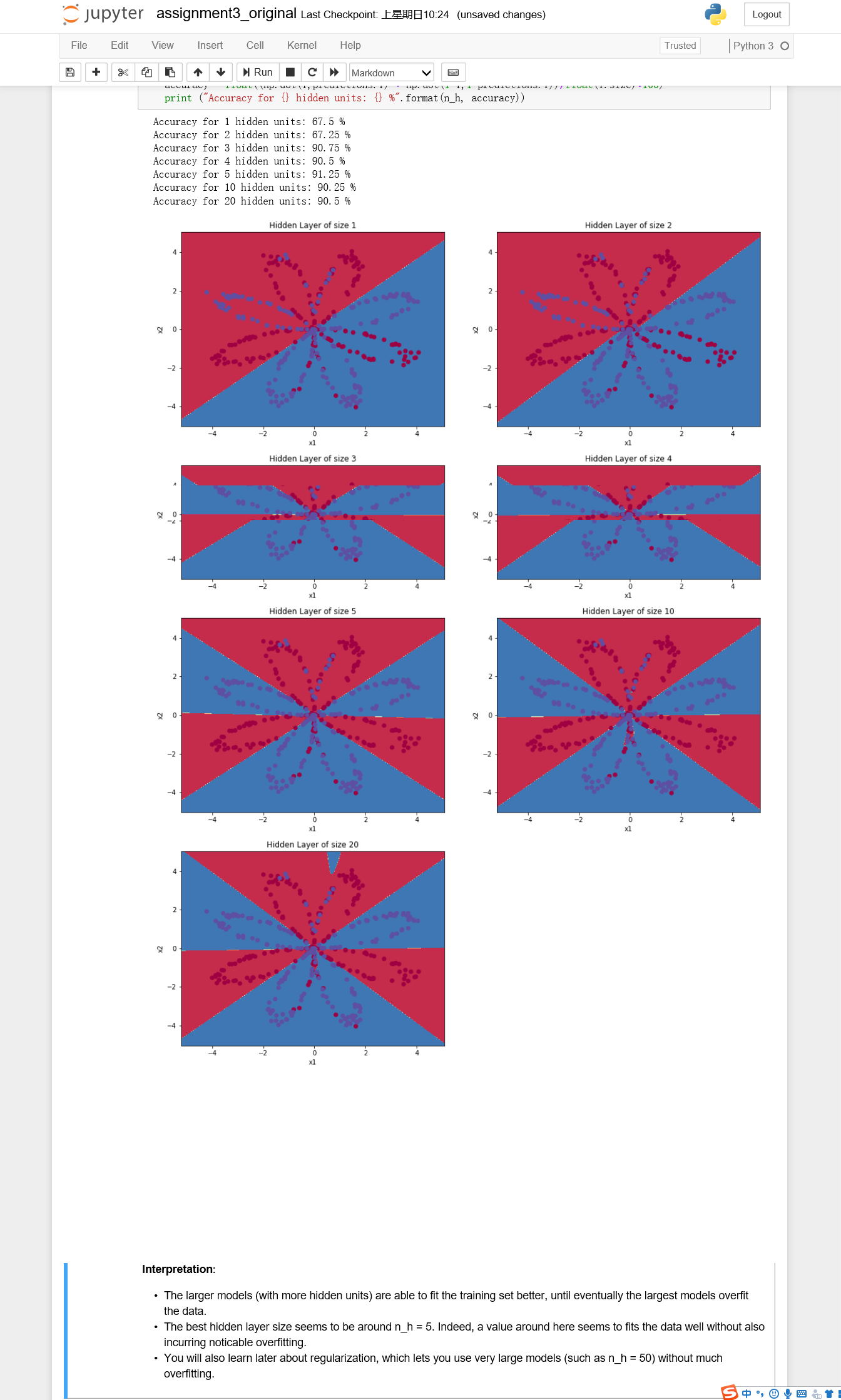
运行以下代码。可能需要1-2分钟。您将观察不同隐藏层大小的模型的不同行为。
# This may take about 2 minutes to run

plt.figure(figsize=(16, 32))
hidden_layer_sizes = [1, 2, 3, 4, 5, 10, 20]
for i, n_h in enumerate(hidden_layer_sizes):
    plt.subplot(5, 2, i+1)
    plt.title('Hidden Layer of size %d' % n_h)
    parameters = nn_model(X, Y, n_h, num_iterations = 5000)
    plot_decision_boundary(lambda x: predict(parameters, x.T), X, Y)
    predictions = predict(parameters, X)
    accuracy = float((np.dot(Y,predictions.T) + np.dot(1-Y,1-predictions.T))/float(Y.size)*100)
    print ("Accuracy for {} hidden units: {} %".format(n_h, accuracy))
结果:
解释:
•较大的模型(隐藏单元更多)能够更好地拟合训练集,直到最终最大的模型对数据进行过拟合。
•最好的隐藏层大小似乎是在n_h = 5左右。实际上,这里的值似乎很适合数据,而不会引起明显的过拟合。
•稍后您还将学习正则化,它可以让您使用非常大的模型(如n_h = 50)而不会过度拟合。
可选的问题:
注意:记得提交作业,但点击右上角的蓝色“提交作业”按钮。
一些可选的/未评分的问题,你可以探索,如果你愿意:
•将tanh激活改为sigmoid激活或ReLU激活会发生什么?
•玩学习率。会发生什么呢?
•如果我们改变数据集会怎么样?(参见下面的第5部分!)
**你已经学会:** -建立一个完整的带有隐含层的神经网络-充分利用非线性单元-实现前向传播和后向传播,训练一个神经网络-看看改变隐含层大小的影响,包括过拟合。
干得漂亮!!!
5) Performance on other datasets (5)其他数据集的性能)
如果需要,可以为以下每个数据集重新运行整个笔记本(减去数据集部分)。
# Datasets
noisy_circles, noisy_moons, blobs, gaussian_quantiles, no_structure = load_extra_datasets()

datasets = {"noisy_circles": noisy_circles,
            "noisy_moons": noisy_moons,
            "blobs": blobs,
            "gaussian_quantiles": gaussian_quantiles}

### START CODE HERE ### (choose your dataset)
dataset = "gaussian_quantiles"
### END CODE HERE ###

X, Y = datasets[dataset]
X, Y = X.T, Y.reshape(1, Y.shape[0])

# make blobs binary
if dataset == "blobs":
    Y = Y%2

# Visualize the data
plt.scatter(X[0, :], X[1, :], c= np.squeeze(Y), s=40, cmap=plt.cm.Spectral);
结果:

祝贺你完成了这个编程任务!
Reference: