为标准正态累积分布函数:
最大绝对误差0.0017。
高斯分布的解析式是 形式,它不可积、没有原函数。但是有时候有需要知道高斯分布任意一段区间的面积,这时就需要用到高斯分布的可积分拟合函数。高斯分布的可积分拟合函数有很多,其中一种形式如下式所示。
我们只需要找到满足上式f(x),那么我们就得到了高斯分布的可积分拟合函数。因为高斯分布具有对称性,所以只考虑x负半轴上的正态分布。
不妨设 是多项式函数,求解的参数包括:多项式中每一项的系数。
求解非线性方程组,瞬间可得很多个可积分的高斯分布。
以下程序尝试了最小二乘法和tensorflow调参两种方法求解非线性方程组。
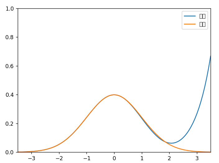
  1 import matplotlib.pyplot as plt
  2 import numpy as np
  3 import tensorflow as tf
  4 from scipy import optimize
  5
  6 """
  7 正态分布的拟合是一个很难调节的神经网络
  8
  9 并非每次运行都能找到合适的解
 10 """
 11
 12
 13 def gauss(xs, mu=0, sigma=1):
 14     return 1 / (sigma * (2 * np.pi) ** 0.5) * np.exp(-(xs - mu) ** 2 / (2 * sigma ** 2))
 15
 16
 17 def my_fun(v):
 18     x = np.linspace(-3.5, 0.1, 1000)
 19     vv = np.empty(len(v) - 1)
 20     for i in range(len(vv)):
 21         vv[i] = v[i + 1] * (i + 1)
 22     y = (
 23         (x.reshape(-1, 1) ** np.arange(len(vv)))
 24         @ vv
 25         * np.exp((x.reshape(-1, 1) ** np.arange(len(v))) @ v)
 26     )
 27     yy = gauss(x)
 28     l = y - yy
 29     print(np.linalg.norm(l))
 30     return l
 31
 32
 33 def draw(v):
 34     x = np.linspace(-3.5, 3.5, 100)
 35     vv = np.empty(len(v) - 1)
 36     for i in range(len(vv)):
 37         vv[i] = v[i + 1] * (i + 1)
 38     y = (
 39         (x.reshape(-1, 1) ** np.arange(len(vv)))
 40         @ vv
 41         * np.exp((x.reshape(-1, 1) ** np.arange(len(v))) @ v)
 42     )
 43     yy = gauss(x)
 44     plt.plot(x, y, label="mine")
 45     plt.plot(x, yy, label="real")
 46     plt.legend()
 47     plt.ylim(0, 1)
 48     plt.xlim(x.min(), x.max())
 49     plt.show()
 50
 51
 52 def print_latex(v):
 53     def pow(y):
 54         if y == 0:
 55             return ""
 56         if y == 1:
 57             return "x"
 58         return f"x^{y}"
 59
 60     s = r"""\frac{1}{\sqrt{2\pi}}e^{-\frac{1}{2}x^2}="""
 61     pre = f"{v[1]:.3f}"
 62     for i in range(1, len(v) - 1):
 63         if v[i + 1] >= 0 and i > 0:
 64             pre += "+"
 65         pre += f"{v[i+1]:.3f} \\times {i+1}{pow(i)}"
 66     post = ""
 67     for i in range(len(v)):
 68         if v[i] >= 0 and i > 0:
 69             post += "+"
 70         post += f"{v[i]:.3f}{pow(i)}"
 71     ss = f"({pre}) \\times e^{{{post}}}"
 72     s = s + ss + r"\\"
 73     print(s)
 74
 75
 76 def get_params_by_tf(n):
 77     x = np.linspace(-3.5, 0.1, 10000)
 78     y = gauss(x)
 79     x_place = tf.placeholder(dtype=tf.float32, shape=(None,))
 80     y_place = tf.placeholder(dtype=tf.float32, shape=(None,))
 81     v = tf.Variable(tf.random.uniform((n,), minval=0, maxval=0.1))
 82     learn_rate = tf.Variable(0.01, trainable=False)
 83     pre = 0
 84     for i in range(n - 1):
 85         pre += x_place ** i * v[i + 1] * (i + 1)
 86     post = 0
 87     for i in range(n):
 88         post += x_place ** i * v[i]
 89     y_output = pre * tf.exp(post)
 90     # lo = tf.reduce_max(tf.abs(y_output - y_place))
 91     # lo = tf.reduce_sum((y_output - y_place) ** 2)
 92     # lo = tf.reduce_sum(tf.abs(y_output - y_place))
 93     lo = tf.linalg.norm(y_output - y_place)
 94     train_op = tf.train.AdamOptimizer(learn_rate).minimize(lo)
 95     with tf.Session() as sess:
 96         sess.run(tf.global_variables_initializer())
 97         last = None
 98         for epoch in range(10000):
 99             _, l = sess.run((train_op, lo), feed_dict={x_place: x, y_place: y})
100             if epoch % 1000 == 0:
101                 rate = sess.run(learn_rate) * 0.99
102                 rate = max(rate, 0.0001)
103                 sess.run(tf.assign(learn_rate, rate))
104                 print(epoch, l)
105                 if last is None:
106                     last = l
107                 else:
108                     if abs(last - l) < 0.0001:
109                         print("last loss", l)
110                         break
111                     last = l
112         res = sess.run(v)
113         return res
114
115
116 def get_param_by_fsolve(n):
117     v = optimize.leastsq(my_fun, np.random.random(n) - 0.5)
118     print("loss", v[1])
119     return v[0]
120
121
122 def wrap_get_param(n):
123     l = 1
124     res = None
125     while l > 0.1:
126         res, l = get_params_by_tf(n)
127     print("last loss", l)
128     return res
129
130
131 v = get_param_by_fsolve(5)
132 print(v)
133 print_latex(v)
134 draw(v)
效果如下: