produce a gradient file using surface elevation data, and plot it using grdimage with topographic "shade"

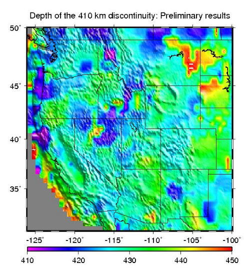
http://web.mst.edu/~sgao/gmtexs/grd/ex05/plot.gmt
#!/bin/csh

/bin/rm tmp.ps tmp.cpt

## Make a basemap of western United States:
psbasemap -R-126.000/-100.000/30.500/50.000 
-JM5 -Ba5f1 -P -X2.0 -Y2 -K >tmp.ps

## Convert the xyz file into GRD file using xyz2grd
awk '{print $1, $2, $4}' data.dat | xyz2grd -R -I0.5 -Gtmp.grd 

## Resample tmp.grd from coarse (0.5 deg.) into finer resolution (0.1 degree) using grdsample. 
#  The output file is tmph.grd. 
grdsample tmp.grd -Gtmph.grd -I0.1 -Ql/0.1 -Lx

## Make a color table
makecpt -Crainbow -T410/450/20 -Z >tmp.cpt

## Make a gradient file out of elevation data to be used as "shade" of the image 
# The output intensity file is tmph.int. The "light" comes from 45 degree (Northeast)
# "N" is for normalization (otherwise the gradients will be too large)

# Cut out the portion of elevation data from a global database
# The output is topo0.grd
grdcut /home/sgao/Dbase/topo1min/data.grd -Gtopo0.grd -R

## Resample it into the same interval as tmph.grd
grdsample topo0.grd -Gtopoh.grd -I0.1 -Ql/0.1 -Lx

## Produce the gradient file. This time I usd -Nt to make a more dramatic shade
grdgradient topoh.grd -Gtopoh.int -A45 -Nt

## Produce the image using the resampled grd file and tmp.int
grdimage tmph.grd -Itopoh.int -Ctmp.cpt -R -J -O -K >>tmp.ps

## Plot the scale bar at the bottom of the plot
psscale -D2.5/-0.4/5.0/0.1h -B10 -Ctmp.cpt -O -K >>tmp.ps


## Overlay with coastlines and political boudnaries
pscoast -R -J -W3 -Df -Na/1/0t10:5_0 -A1000 -O -K -B  >>tmp.ps


## Add a title
pstext -R -J -O -N  <<END>>tmp.ps
-113 51 15 0 0 6 Depth of the 410 km discontinuity: Preliminary results
END

## Convert tmp.ps into a JPG file:

ps2jpeg100 tmp.ps