tensorflow笔记（二）之构造一个简单的神经网络

tensorflow笔记（二）之构造一个简单的神经网络

版权声明：本文为博主原创文章，转载请指明转载地址

http://www.cnblogs.com/fydeblog/p/7425200.html

前言

这篇博客将一步步构建一个tensorflow的神经网络去拟合曲线，并将误差和结果可视化。博客的末尾会放本篇博客的jupyter notebook，可以下载自己调试调试。

实践——构造神经网络

本次构造的神经网络是要拟合一个二次曲线，神经网络的输入层是一个特征，即只有一个神经元，隐藏层有10个特征，即有10个神经元，输出为一个神经元，总结起来就是1—10—1的结构，如果没有神经网络结构的朋友，还请去补一补

首先我们先导入要用到的模块

import tensorflow as tf 
import numpy as np
import matplotlib.pyplot as plt

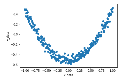
然后我们先构造出原始数据，并画出它的图形（为了更加符合实际，我们会加一些噪声）

x_data = np.linspace(-1,1,300) [:, np.newaxis]   # [:,np.newaxis] make row vector transform column vector
noise = np.random.normal(0, 0.05, x_data.shape) 
y_data = np.square(x_data) - 0.5 + noise

x_data是一个范围-1到1，以300分之2等份的列向量，noise的shape与x_data一样，值属于正态分布，0到0.05之间，y_data则是x_data的平方，减0.5，加噪声

fig=plt.figure()
ax = fig.add_subplot(1,1,1)
ax.scatter(x_data,y_data)
plt.xlabel('x_data')
plt.ylabel('y_data')
plt.show()

现在我们先写一个添加神经网络层的函数，函数名为add_nn_layer

def add_nn_layer(inputs, in_size, out_size, activation_function=None):
    Weights = tf.Variable(tf.random_normal([in_size, out_size]))
    biases = tf.Variable(tf.zeros([1, out_size]) + 0.1)  
    Wx_plus_b = tf.matmul(inputs, Weights) + biases
    if activation_function is None:
        outputs = Wx_plus_b
    else:
        outputs = activation_function(Wx_plus_b)
    return outputs

神经网络的基本构造是要有输入，还要有输入映射到下一层的权重和偏差，最后神经元还有一个激活函数（这个有没有看需求），控制输出
我们上面讲到这个神经网络的结构是1—10—1，所以要添加两个层，一层是从输入层到隐藏层，另一层是隐藏层到输出层。
从输入层到隐藏层，1—10，输入是300x1的向量，到第二层则是300x10，权重则是1x10，偏差的shape与输出相同
从隐藏层到输出层，10—1，输入是300x10的向量，输出是300x1，可见权重是10x1，偏差的shape与输出相同
由此可以知道上面函数中各种变量的构造原因，简单说神经网络的构造就是输入乘以权重加上偏差，进入神经元的激活函数，然后输出

接下来我们开始写其他代码

xs = tf.placeholder(tf.float32, [None, 1])
ys = tf.placeholder(tf.float32, [None, 1])

tf.placeholder函数是一个非常重要的函数，以后用到它的次数会非常多，它表示占位符，相应的值会在sess.run里面feed进去，这样处理会非常灵活，大部分的学习都是分批的，不是一次传入，占位符满足这种需求
这里的xs和ys都是列向量，列数为1，行数不确定，feed的输入行数是多少就是多少

# add hidden layer
l1 = add_nn_layer(xs, 1, 10, activation_function=tf.nn.relu)
# add output layer
prediction = add_nn_layer(l1, 10, 1, activation_function=None)

这里隐藏层的激活函数用的是tf.nn.relu，relu全名是修正线性单元，详细请参考wiki（https://en.wikipedia.org/wiki/Rectifier_(neural_networks) ），它的性质简单的说就是输入神经元的数据大于0则等于自身，小于0则等于0，使用它更符合神经网络的性质，即有抑制区域和激活区域，我试了没加激活函数和sigmoid激活函数，效果要比用relu差许多，你们可以试试。

#compute loss
loss = tf.reduce_mean(tf.reduce_sum(tf.square(ys - prediction),reduction_indices=[1]))
# creat train op，then we can sess.run(train)  to minimize loss
train = tf.train.GradientDescentOptimizer(0.1).minimize(loss)

# creat init 
init = tf.global_variables_initializer()

# creat a Session
sess = tf.Session()

# system initialize
sess.run(init)

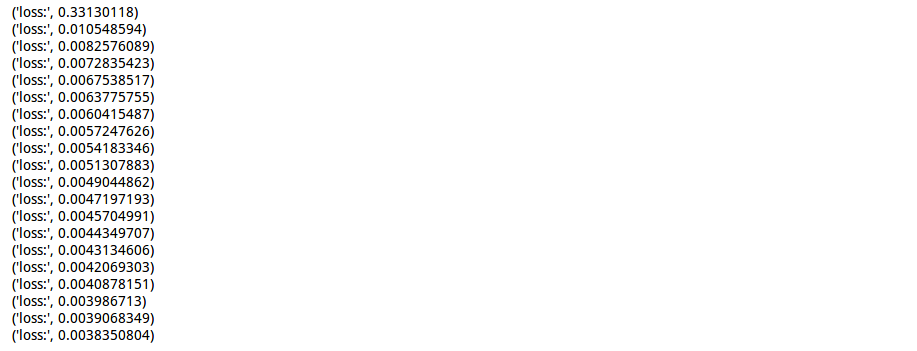
# training 
for i in range(1000):
    sess.run(train, feed_dict={xs: x_data, ys: y_data})
    prediction_value = sess.run(prediction, feed_dict={xs: x_data})
    if i % 50 == 0:
        # to see the step improvement
        print('loss:',sess.run(loss, feed_dict={xs: x_data, ys: y_data}))

最后我们来看一下拟合的效果

fig=plt.figure()
bx = fig.add_subplot(1,1,1)
bx.scatter(x_data,y_data)
bx.plot(x_data,prediction_value,'g-',lw=6)
plt.xlabel('x_data')
plt.ylabel('y_data')
plt.show()

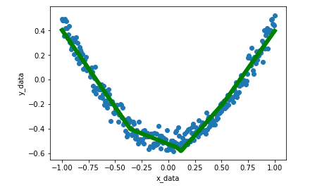
可见拟合的不错

结尾

下一个笔记将讲讲tensorboard的一些用法，敬请期待！

百度云链接: https://pan.baidu.com/s/1skAfUGH 密码: qw1g