根据以上两篇的分析,下面我们还要对数据进行处理,观察Age和Fare两个属性,乘客的数值变化幅度较大!根据逻辑回归和梯度下降的了解,如果属性值之间scale差距较大,将对收敛速度造成较大影响,甚至不收敛!因此,我们需要运用scikit-learn里面的preprocessing模块对Age和Fare两个属性做一个scaling,即将其数值转化为[-1,1]范围内。
1 # 接下来我们将一些变化幅度较大的特征化到[-1,1]之内,这样可以加速logistic regression的收敛
2 import sklearn.preprocessing as preprocessing
3 scaler = preprocessing.StandardScaler()
4 age_scale_param = scaler.fit(df['Age'])
5 df['Age_scaled'] = scaler.fit_transform(df['Age'],age_scale_param)
6 fare_scale_param = scaler.fit(df['Fare'])
7 df['Fare_scaled'] = scaler.fit_transform(df['Fare'],fare_scale_param)
8 print(df)
|
|
PassengerId |
Survived |
Age |
SibSp |
Parch |
Fare |
Cabin_No |
Cabin_Yes |
Embarked_C |
Embarked_Q |
Embarked_S |
Sex_female |
Sex_male |
Pclass_1 |
Pclass_2 |
Pclass_3 |
Age_scaled |
Fare_scaled |
|
0 |
1 |
0 |
22.000000 |
1 |
0 |
7.2500 |
1 |
0 |
0 |
0 |
1 |
0 |
1 |
0 |
0 |
1 |
-0.561417 |
-0.502445 |
|
1 |
2 |
1 |
38.000000 |
1 |
0 |
71.2833 |
0 |
1 |
1 |
0 |
0 |
1 |
0 |
1 |
0 |
0 |
0.613177 |
0.786845 |
|
2 |
3 |
1 |
26.000000 |
0 |
0 |
7.9250 |
1 |
0 |
0 |
0 |
1 |
1 |
0 |
0 |
0 |
1 |
-0.267768 |
-0.488854 |
|
3 |
4 |
1 |
35.000000 |
1 |
0 |
53.1000 |
0 |
1 |
0 |
0 |
1 |
1 |
0 |
1 |
0 |
0 |
0.392941 |
0.420730 |
|
4 |
5 |
0 |
35.000000 |
0 |
0 |
8.0500 |
1 |
0 |
0 |
0 |
1 |
0 |
1 |
0 |
0 |
1 |
0.392941 |
-0.486337 |
|
5 |
6 |
0 |
23.828953 |
0 |
0 |
8.4583 |
1 |
0 |
0 |
1 |
0 |
0 |
1 |
0 |
0 |
1 |
-0.427149 |
-0.478116 |
|
6 |
7 |
0 |
54.000000 |
0 |
0 |
51.8625 |
0 |
1 |
0 |
0 |
1 |
0 |
1 |
1 |
0 |
0 |
1.787771 |
0.395814 |
|
7 |
8 |
0 |
2.000000 |
3 |
1 |
21.0750 |
1 |
0 |
0 |
0 |
1 |
0 |
1 |
0 |
0 |
1 |
-2.029659 |
-0.224083 |
|
8 |
9 |
1 |
27.000000 |
0 |
2 |
11.1333 |
1 |
0 |
0 |
0 |
1 |
1 |
0 |
0 |
0 |
1 |
-0.194356 |
-0.424256 |
|
9 |
10 |
1 |
14.000000 |
1 |
0 |
30.0708 |
1 |
0 |
1 |
0 |
0 |
1 |
0 |
0 |
1 |
0 |
-1.148714 |
-0.042956 |
|
10 |
11 |
1 |
4.000000 |
1 |
1 |
16.7000 |
0 |
1 |
0 |
0 |
1 |
1 |
0 |
0 |
0 |
1 |
-1.882835 |
-0.312172 |
|
11 |
12 |
1 |
58.000000 |
0 |
0 |
26.5500 |
0 |
1 |
0 |
0 |
1 |
1 |
0 |
1 |
0 |
0 |
2.081420 |
-0.113846 |
|
12 |
13 |
0 |
20.000000 |
0 |
0 |
8.0500 |
1 |
0 |
0 |
0 |
1 |
0 |
1 |
0 |
0 |
1 |
-0.708241 |
-0.486337 |
|
13 |
14 |
0 |
39.000000 |
1 |
5 |
31.2750 |
1 |
0 |
0 |
0 |
1 |
0 |
1 |
0 |
0 |
1 |
0.686589 |
-0.018709 |
|
14 |
15 |
0 |
14.000000 |
0 |
0 |
7.8542 |
1 |
0 |
0 |
0 |
1 |
1 |
0 |
0 |
0 |
1 |
-1.148714 |
-0.490280 |
|
15 |
16 |
1 |
55.000000 |
0 |
0 |
16.0000 |
1 |
0 |
0 |
0 |
1 |
1 |
0 |
0 |
1 |
0 |
1.861183 |
-0.326267 |
|
16 |
17 |
0 |
2.000000 |
4 |
1 |
29.1250 |
1 |
0 |
0 |
1 |
0 |
0 |
1 |
0 |
0 |
1 |
-2.029659 |
-0.061999 |
|
17 |
18 |
1 |
32.066493 |
0 |
0 |
13.0000 |
1 |
0 |
0 |
0 |
1 |
0 |
1 |
0 |
1 |
0 |
0.177586 |
-0.386671 |
|
18 |
19 |
0 |
31.000000 |
1 |
0 |
18.0000 |
1 |
0 |
0 |
0 |
1 |
1 |
0 |
0 |
0 |
1 |
0.099292 |
-0.285997 |
|
19 |
20 |
1 |
29.518205 |
0 |
0 |
7.2250 |
1 |
0 |
1 |
0 |
0 |
1 |
0 |
0 |
0 |
1 |
-0.009489 |
-0.502949 |
|
20 |
21 |
0 |
35.000000 |
0 |
0 |
26.0000 |
1 |
0 |
0 |
0 |
1 |
0 |
1 |
0 |
1 |
0 |
0.392941 |
-0.124920 |
|
21 |
22 |
1 |
34.000000 |
0 |
0 |
13.0000 |
0 |
1 |
0 |
0 |
1 |
0 |
1 |
0 |
1 |
0 |
0.319529 |
-0.386671 |
|
22 |
23 |
1 |
15.000000 |
0 |
0 |
8.0292 |
1 |
0 |
0 |
1 |
0 |
1 |
0 |
0 |
0 |
1 |
-1.075302 |
-0.486756 |
|
23 |
24 |
1 |
28.000000 |
0 |
0 |
35.5000 |
0 |
1 |
0 |
0 |
1 |
0 |
1 |
1 |
0 |
0 |
-0.120944 |
0.066360 |
|
24 |
25 |
0 |
8.000000 |
3 |
1 |
21.0750 |
1 |
0 |
0 |
0 |
1 |
1 |
0 |
0 |
0 |
1 |
-1.589186 |
-0.224083 |
|
25 |
26 |
1 |
38.000000 |
1 |
5 |
31.3875 |
1 |
0 |
0 |
0 |
1 |
1 |
0 |
0 |
0 |
1 |
0.613177 |
-0.016444 |
|
26 |
27 |
0 |
29.518205 |
0 |
0 |
7.2250 |
1 |
0 |
1 |
0 |
0 |
0 |
1 |
0 |
0 |
1 |
-0.009489 |
-0.502949 |
|
27 |
28 |
0 |
19.000000 |
3 |
2 |
263.0000 |
0 |
1 |
0 |
0 |
1 |
0 |
1 |
1 |
0 |
0 |
-0.781653 |
4.647001 |
|
28 |
29 |
1 |
22.380113 |
0 |
0 |
7.8792 |
1 |
0 |
0 |
1 |
0 |
1 |
0 |
0 |
0 |
1 |
-0.533512 |
-0.489776 |
|
29 |
30 |
0 |
27.947206 |
0 |
0 |
7.8958 |
1 |
0 |
0 |
0 |
1 |
0 |
1 |
0 |
0 |
1 |
-0.124820 |
-0.489442 |
|
... |
... |
... |
... |
... |
... |
... |
... |
... |
... |
... |
... |
... |
... |
... |
... |
... |
... |
... |
|
861 |
862 |
0 |
21.000000 |
1 |
0 |
11.5000 |
1 |
0 |
0 |
0 |
1 |
0 |
1 |
0 |
1 |
0 |
-0.634829 |
-0.416873 |
|
862 |
863 |
1 |
48.000000 |
0 |
0 |
25.9292 |
0 |
1 |
0 |
0 |
1 |
1 |
0 |
1 |
0 |
0 |
1.347299 |
-0.126345 |
|
863 |
864 |
0 |
10.888325 |
8 |
2 |
69.5500 |
1 |
0 |
0 |
0 |
1 |
1 |
0 |
0 |
0 |
1 |
-1.377148 |
0.751946 |
|
864 |
865 |
0 |
24.000000 |
0 |
0 |
13.0000 |
1 |
0 |
0 |
0 |
1 |
0 |
1 |
0 |
1 |
0 |
-0.414592 |
-0.386671 |
|
865 |
866 |
1 |
42.000000 |
0 |
0 |
13.0000 |
1 |
0 |
0 |
0 |
1 |
1 |
0 |
0 |
1 |
0 |
0.906826 |
-0.386671 |
|
866 |
867 |
1 |
27.000000 |
1 |
0 |
13.8583 |
1 |
0 |
1 |
0 |
0 |
1 |
0 |
0 |
1 |
0 |
-0.194356 |
-0.369389 |
|
867 |
868 |
0 |
31.000000 |
0 |
0 |
50.4958 |
0 |
1 |
0 |
0 |
1 |
0 |
1 |
1 |
0 |
0 |
0.099292 |
0.368295 |
|
868 |
869 |
0 |
25.977889 |
0 |
0 |
9.5000 |
1 |
0 |
0 |
0 |
1 |
0 |
1 |
0 |
0 |
1 |
-0.269391 |
-0.457142 |
|
869 |
870 |
1 |
4.000000 |
1 |
1 |
11.1333 |
1 |
0 |
0 |
0 |
1 |
0 |
1 |
0 |
0 |
1 |
-1.882835 |
-0.424256 |
|
870 |
871 |
0 |
26.000000 |
0 |
0 |
7.8958 |
1 |
0 |
0 |
0 |
1 |
0 |
1 |
0 |
0 |
1 |
-0.267768 |
-0.489442 |
|
871 |
872 |
1 |
47.000000 |
1 |
1 |
52.5542 |
0 |
1 |
0 |
0 |
1 |
1 |
0 |
1 |
0 |
0 |
1.273886 |
0.409741 |
|
872 |
873 |
0 |
33.000000 |
0 |
0 |
5.0000 |
0 |
1 |
0 |
0 |
1 |
0 |
1 |
1 |
0 |
0 |
0.246117 |
-0.547748 |
|
873 |
874 |
0 |
47.000000 |
0 |
0 |
9.0000 |
1 |
0 |
0 |
0 |
1 |
0 |
1 |
0 |
0 |
1 |
1.273886 |
-0.467209 |
|
874 |
875 |
1 |
28.000000 |
1 |
0 |
24.0000 |
1 |
0 |
1 |
0 |
0 |
1 |
0 |
0 |
1 |
0 |
-0.120944 |
-0.165189 |
|
875 |
876 |
1 |
15.000000 |
0 |
0 |
7.2250 |
1 |
0 |
1 |
0 |
0 |
1 |
0 |
0 |
0 |
1 |
-1.075302 |
-0.502949 |
|
876 |
877 |
0 |
20.000000 |
0 |
0 |
9.8458 |
1 |
0 |
0 |
0 |
1 |
0 |
1 |
0 |
0 |
1 |
-0.708241 |
-0.450180 |
|
877 |
878 |
0 |
19.000000 |
0 |
0 |
7.8958 |
1 |
0 |
0 |
0 |
1 |
0 |
1 |
0 |
0 |
1 |
-0.781653 |
-0.489442 |
|
878 |
879 |
0 |
27.947206 |
0 |
0 |
7.8958 |
1 |
0 |
0 |
0 |
1 |
0 |
1 |
0 |
0 |
1 |
-0.124820 |
-0.489442 |
|
879 |
880 |
1 |
56.000000 |
0 |
1 |
83.1583 |
0 |
1 |
1 |
0 |
0 |
1 |
0 |
1 |
0 |
0 |
1.934596 |
1.025945 |
|
880 |
881 |
1 |
25.000000 |
0 |
1 |
26.0000 |
1 |
0 |
0 |
0 |
1 |
1 |
0 |
0 |
1 |
0 |
-0.341180 |
-0.124920 |
|
881 |
882 |
0 |
33.000000 |
0 |
0 |
7.8958 |
1 |
0 |
0 |
0 |
1 |
0 |
1 |
0 |
0 |
1 |
0.246117 |
-0.489442 |
|
882 |
883 |
0 |
22.000000 |
0 |
0 |
10.5167 |
1 |
0 |
0 |
0 |
1 |
1 |
0 |
0 |
0 |
1 |
-0.561417 |
-0.436671 |
|
883 |
884 |
0 |
28.000000 |
0 |
0 |
10.5000 |
1 |
0 |
0 |
0 |
1 |
0 |
1 |
0 |
1 |
0 |
-0.120944 |
-0.437007 |
|
884 |
885 |
0 |
25.000000 |
0 |
0 |
7.0500 |
1 |
0 |
0 |
0 |
1 |
0 |
1 |
0 |
0 |
1 |
-0.341180 |
-0.506472 |
|
885 |
886 |
0 |
39.000000 |
0 |
5 |
29.1250 |
1 |
0 |
0 |
1 |
0 |
1 |
0 |
0 |
0 |
1 |
0.686589 |
-0.061999 |
|
886 |
887 |
0 |
27.000000 |
0 |
0 |
13.0000 |
1 |
0 |
0 |
0 |
1 |
0 |
1 |
0 |
1 |
0 |
-0.194356 |
-0.386671 |
|
887 |
888 |
1 |
19.000000 |
0 |
0 |
30.0000 |
0 |
1 |
0 |
0 |
1 |
1 |
0 |
1 |
0 |
0 |
-0.781653 |
-0.044381 |
|
888 |
889 |
0 |
16.232379 |
1 |
2 |
23.4500 |
1 |
0 |
0 |
0 |
1 |
1 |
0 |
0 |
0 |
1 |
-0.984830 |
-0.176263 |
|
889 |
890 |
1 |
26.000000 |
0 |
0 |
30.0000 |
0 |
1 |
1 |
0 |
0 |
0 |
1 |
1 |
0 |
0 |
-0.267768 |
-0.044381 |
|
890 |
891 |
0 |
32.000000 |
0 |
0 |
7.7500 |
1 |
0 |
0 |
1 |
0 |
0 |
1 |
0 |
0 |
1 |
0.172705 |
-0.492378 |
891 rows × 18 columns
接下来我们把需要的feature字段取出来,转成numpy格式,使用scikit-learn中的LogisticRegression建模。
1 from sklearn import linear_model
2 train_df = df.filter(regex='Survived|Age_.*|SibSp|Parch|Fare_.*|Cabin_.*|Embarked_.*|Sex_.*|Pclass_.*')
3 train_np = train_df.as_matrix()
4 y = train_np[:,0]
5 X = train_np[:,1:]
6 clf = linear_model.LogisticRegression(C=1.0,penalty='l1',tol=1e-6)
7 clf.fit(X,y)
8 print(clf)
接下来我们需要对测试数据集和训练数据集做一样的操作
 1 # #首先用同样的RandomForestRegressor模型填上丢失的年龄
 2 data_test = pd.read_csv("test.csv")
 3 data_test.loc[ (data_test.Fare.isnull()), 'Fare' ] = 0
 4
 5 tmp_df = data_test[['Age','Fare', 'Parch', 'SibSp', 'Pclass']]
 6 null_age = tmp_df[data_test.Age.isnull()].as_matrix()
 7 # 根据特征属性X预测年龄并补上
 8 X = null_age[:, 1:]
 9 predictedAges = rfr.predict(X)
10 data_test.loc[ (data_test.Age.isnull()), 'Age' ] = predictedAges
11
12 data_test = set_Cabin_type(data_test)
13 dummies_Cabin = pd.get_dummies(data_test['Cabin'], prefix= 'Cabin')
14 dummies_Embarked = pd.get_dummies(data_test['Embarked'], prefix= 'Embarked')
15 dummies_Sex = pd.get_dummies(data_test['Sex'], prefix= 'Sex')
16 dummies_Pclass = pd.get_dummies(data_test['Pclass'], prefix= 'Pclass')
17
18
19 df_test = pd.concat([data_test, dummies_Cabin, dummies_Embarked, dummies_Sex, dummies_Pclass], axis=1)
20 df_test.drop(['Pclass', 'Name', 'Sex', 'Ticket', 'Cabin', 'Embarked'], axis=1, inplace=True)
21 df_test['Age_scaled'] = scaler.fit_transform(df_test['Age'], age_scale_param)
22 df_test['Fare_scaled'] = scaler.fit_transform(df_test['Fare'], fare_scale_param)
23
24 test = df_test.filter(regex='Age_.*|SibSp|Parch|Fare_.*|Cabin_.*|Embarked_.*|Sex_.*|Pclass_.*')
25 predictions = clf.predict(test)
26 result = pd.DataFrame({'PassengerId':data_test['PassengerId'].as_matrix(), 'Survived':predictions.astype(np.int32)})
27 result.to_csv("logistic_regression_predictions.csv", index=False)
最后我们将预测的结果保存在logistic_regression_predictions.csv文件里。到这里只是简单分析过后的一个baseline系统。
下面要判定一下当前模型所处状态(欠拟合或者过拟合)
这里面有个问题,前面不断地做特征工程,产生的特征越来越多,用这些特征来训练模型,会对训练集拟合得越来越好,同时也可能在逐步丧失泛化能力,从而在待测数据上表现不佳,也就是发生过拟合问题。
从另一个角度上说,如果模型在待测数据上表现不佳,除掉上述说的过拟合问题,有时候也存在欠拟合问题,也就是说在训练集上拟合的结果也不好。
对于过拟合和欠拟合,有两种优化方式:
1.过拟合
1)做一个feature selection,选较好的feature的subset来做training
2)提供更多的数据,从而弥补原始数据偏差,从而学习到的模型更准确
3)采用正则化,正则化方法包括L0正则、L1正则和L2正则,而正则一般是在目标函数之后加上对于的范数。但是在机器学习中一般使用L2正则。
2.欠拟合
1)添加其他特征项,有时候我们模型出现欠拟合的时候是因为特征项不够导致的,可以添加其他特征项来很好地解决。例如,“组合”、“泛化”、“相关性”三类特征是特征添加的重要手段。
2)添加多项式特征,这个在机器学习算法里面用的很普遍,例如将线性模型通过添加二次项或者三次项使模型泛化能力更强。
3)减少正则化参数,正则化的目的是用来防止过拟合的,但是现在模型出现了欠拟合,则需要减少正则化参数。
scikit-learn里面的learning curve可以帮助我们判定模型现在所处的状态。这里我们画一下最先得到的baseline model的learning curve。
 1 import numpy as np
 2 import matplotlib.pyplot as plt
 3 from sklearn.learning_curve import learning_curve
 4
 5 #用sklearn的learning_curve得到training_score和cv_score,使用matplotlib画出learning curve
 6
 7 def plot_learning_curve(estimator,title,X,y,ylim=None,cv=None,n_jobs=1,train_sizes=np.linspace(.05,1.,20),verbose=0,plot=True):
 8     """
 9        画出data在某模型上的learning curve.
10        参数解释
11        ----------
12        estimator : 你用的分类器。
13        title : 表格的标题。
14        X : 输入的feature,numpy类型
15        y : 输入的target vector
16        ylim : tuple格式的(ymin, ymax), 设定图像中纵坐标的最低点和最高点
17        cv : 做cross-validation的时候,数据分成的份数,其中一份作为cv集,其余n-1份作为training(默认为3份)
18        n_jobs : 并行的的任务数(默认1)
19        """
20     train_sizes, train_scores, test_scores = learning_curve(
21         estimator, X, y, cv=cv, n_jobs=n_jobs, train_sizes=train_sizes, verbose=verbose)
22
23     train_scores_mean = np.mean(train_scores, axis=1)
24     train_scores_std = np.std(train_scores, axis=1)
25     test_scores_mean = np.mean(test_scores, axis=1)
26     test_scores_std = np.std(test_scores, axis=1)
27
28     if plot:
29         plt.figure()
30         plt.title(title)
31         if ylim is not None:
32             plt.ylim(*ylim)
33         plt.xlabel('train_sample')
34         plt.ylabel('score')
35         plt.gca().invert_yaxis()
36         plt.grid()
37
38         plt.fill_between(train_sizes, train_scores_mean - train_scores_std, train_scores_mean + train_scores_std,
39                          alpha=0.1, color="b")
40         plt.fill_between(train_sizes, test_scores_mean - test_scores_std, test_scores_mean + test_scores_std,
41                          alpha=0.1, color="r")
42         plt.plot(train_sizes, train_scores_mean, 'o-', color="b", label="train_score")
43         plt.plot(train_sizes, test_scores_mean, 'o-', color="r", label="cross_validation_score")
44
45         plt.legend(loc='best')
46         plt.draw()
47         plt.gca().invert_yaxis()
48         plt.show()
49
50     midpoint = ((train_scores_mean[-1] + train_scores_std[-1]) + (test_scores_mean[-1] - test_scores_std[-1])) / 2
51     diff = (train_scores_mean[-1] + train_scores_std[-1]) - (test_scores_mean[-1] - test_scores_std[-1])
52     return midpoint, diff
53
54 plot_learning_curve(clf, u"学习曲线", X, y)
结果如下(0.80656968448540245, 0.018258876711338634)
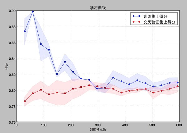
从得到的结果来看,尽管learn——curve没有理论推导的光滑,但是仍可以看出,训练集和交叉验证集上的得分曲线走势还是符合预期的。
目前的曲线来看,我们的model并不处于overfitting的状态(overfitting的表现一般是训练集得分高,交叉验证集得分低很多,中间的gap比较大)。因此我们可以再做些feature engineering的工作,添加一些新的特征或者组合特征到模型中。