logistic回归模型
logistic回归就是将线性回归模型的结果输入一个Sigmoid函数,将回归结果映射到0-1之间,表示类别“1”的概率。
线性回归表达式:zi = w*xi + b
Sigmoid函数:yi = 1/(1 + e-zi) ,zi为自变量,yi为因变量,e为自然常数
将yi = 1视为正例的可能性:a = P(yi = 1|xi) = 1/(1 + e-(w*xi + b)) = ew*xi + b / (1 + ew*xi + b)
将yi = 0视为正例的可能性:b = P(yi = 0|xi) = 1 - P(yi = 1|xi) = 1 / (1 + ew*xi + b)
定义两者比值的“概率”,对其取对数得到“对数概率”可得:ln(a/b) = w*xi + b
logistic回归的本质就是用线性回归的预测结果w*xi + b去逼近真实标记的对数概率ln(y/(y1-y)) ,所以logistic回归被称为“对数概率回归”。
logistic回归的sklearn实现
logistic模型:
from sklearn.linear_model import LogisticRegression
LogisticRegression(penalty='l2' ,
                   c = 1.0 ,
                   fit_intercept=True ,
                   class_weight=None ,
                   solver='liblinear' ,
                   max_iter=100 ,
                   tol=0.0001 ,
                   multi_class='ovr' ,
                   dual=False ,
                   warm_start=False ,
                   n_jobs=-1)
参数:
pemalty:指定似然函数中加入正则化项,默认为l2,表示添加L2正则项,也可以使用l1,表示添加L1正则项
c:指定正则项的权重,是正则化项惩罚系数的倒数,所以c越小,正则化惩罚项就越大
fit_intercept:选择是否计算偏置常数b,默认为True ,表示计算
class_weight:指定各类别的权重,默认为None,当样本很不均衡时使用balanced
solver:指定求解最优化问题的算法,默认为liblinear ,适用于数据集较小的情况。当数据集较大的时候可以使用sag,随机梯度下降法。还可以使用newton-cg(牛顿法)和lbfgs(拟牛顿法)。sag、newton-cg、lbfgs只适用于penalty = ‘l2‘的时候
max_iter:设定最大迭代次数,默认为100次
tol:设定判断迭代收斂函数,默认为0.0001
multi_class:指定多分类的策略,默认为ovr ,表示采用one-vs-rest,一对其他策略。选择multinomial ,表示直接采用多项Logistic回归策略
dual:选择是否采用对偶方式求解,默认为False。只有penalty = ‘l2‘ 且solver = ‘liblinear’时才存在对偶形式
warm_start:设定是否使用前一次训练的结果继续训练,默认为False,表示每次从头开始训练
n_jobs:略.....
属性:
coef_:用于输出线性回归模型的权重向量w
intercept_:用于输出线性回归模型的偏置常数b
n_iter_:用于输出实际迭代的次数
方法:
fit(X_train ,y_train):进行模型训练
score(X_test ,y_test):返回模型在测试集上的预测准确率
predict(X):用训练好的模型来预测待预测数据集X,返回数据为预测集对应的预测结果yˆ
predict_proba(X):返回一个数组,数组元素依次为预测集X属于各个类别的概率
predict_log_proba(X):返回一个数组,数组的元素依次是预测集X属于各个类别的对数概率
logistic之泰坦尼克号生存分析
数据:链接: https://pan.baidu.com/s/1CP-eDuvrgVxRGXtsbpkl_Q 密码: stcq
import numpy as np
import pandas as pd
import matplotlib.pyplot as plt
import seaborn as sns
import pycard as pc

train = pd.read_clipboard()
test = pd.read_clipboard()
sub = pd.read_clipboard()
test = test.merge(sub ,how = 'left' ,on = 'PassengerId')
"""
数据集各字段的含义
PassengerId 乘客编号
Survived 是否幸存
Pclass 船票等级
Name 乘客姓名
Sex 乘客性别
SibSp 亲戚数量(兄妹、配偶数)
Parch 亲戚数量(父母、子女数)
Ticket 船票号码
Fare 船票价格
Cabin 船舱
Embarked 登录港口
"""
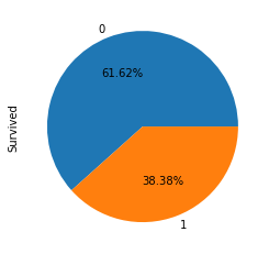
1、查看生还者比例
train['Survived'].value_counts().plot.pie(autopct='%0.2f%%')
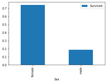
2、查看性别在幸存者之中的占比
train[['Sex','Survived']].groupby(['Sex']).mean().plot.bar()
3、查看船票等级在幸存者中的比例
train[['Pclass','Survived']].groupby(['Pclass']).mean().plot.bar()

4、按照年龄,将乘客划分为儿童、少年、成年和老年,分析四个群体的生还情况
bins = [0, 12, 18, 65, 100]
train['Age_group'] = pd.cut(train['Age'], bins)
by_age = train.groupby('Age_group')['Survived'].mean()
by_age.plot.bar()

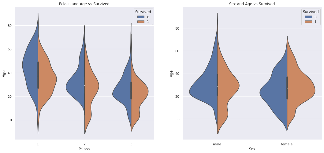
5、查看性别、船票等级幸存者在年龄段的分布
fig, ax = plt.subplots(1, 2, figsize = (18, 8))
sns.violinplot("Pclass", "Age", hue="Survived", data=train, split=True, ax=ax[0])
ax[0].set_title('Pclass and Age vs Survived')
#ax[0].set_yticks(range(0, 110, 10))
sns.violinplot("Sex", "Age", hue="Survived", data=train, split=True, ax=ax[1])
ax[1].set_title('Sex and Age vs Survived')
#ax[1].set_yticks(range(0, 110, 10))
plt.show()
6、查看缺失值的情况,并且使用随机森林对年龄进行填充,对其他缺失进行众数填充
#查看缺失值的情况
test.isnull().sum()

train.Embarked[train.Embarked.isnull()] = train.Embarked.dropna().mode().values#众数填充
test.Embarked[test.Embarked.isnull()] = test.Embarked.dropna().mode().values#众数填充

test.Fare[test.Fare.isnull()] = test.Fare.dropna().mode().values#众数填充
from sklearn.ensemble import RandomForestRegressor
age_df = train[['Age','Survived','Fare', 'Parch', 'SibSp', 'Pclass']]
age_df_notnull = age_df.loc[(train['Age'].notnull())] #选择age不为空的行
age_df_isnull = age_df.loc[(train['Age'].isnull())]

X = age_df_notnull.values[:,1:]

Y = age_df_notnull.values[:,0]

RFR = RandomForestRegressor(n_estimators=1000, n_jobs=-1)
RFR.fit(X,Y)
predictAges = RFR.predict(age_df_isnull.values[:,1:])
train.loc[train['Age'].isnull(), ['Age']]= predictAges
age_df = test[['Age','Survived','Fare', 'Parch', 'SibSp', 'Pclass']]
age_df_notnull = age_df.loc[(test['Age'].notnull())] #选择age不为空的行
age_df_isnull = age_df.loc[(test['Age'].isnull())]

X = age_df_notnull.values[:,1:]

Y = age_df_notnull.values[:,0]

RFR = RandomForestRegressor(n_estimators=1000, n_jobs=-1)
RFR.fit(X,Y)
predictAges = RFR.predict(age_df_isnull.values[:,1:])
test.loc[test['Age'].isnull(), ['Age']]= predictAges
7、数据离散化
# 因为费用最偏严重,此处使用等深分箱
S1 = pd.qcut(train['Fare'], q=5, labels=[0, 1, 2, 3, 4])
S2 = pd.qcut(test['Fare'], q=5, labels=[0, 1, 2, 3, 4])
# pd.cut(train_data['Fare'], bins=5, labels=[0,1,2,3,4])
train['Fare'] = S1
test['Fare'] = S2
train.head(10)

# 年龄值有很多缺失值,并且我们把确实值填为了均值,所以用等深
pd.qcut(train['Age'], q=5, labels=[0,1,2,3,4]).value_counts()
S3 = pd.qcut(train['Age'], q=5, labels=[0, 1, 2, 3, 4])
S4 = pd.qcut(test['Age'], q=5, labels=[0, 1, 2, 3, 4])
# pd.cut(train_data['Fare'], bins=5, labels=[0,1,2,3,4])
train['Age'] = S3
test['Age'] = S4
train.head(10)
8、类别变量进行数值化处理
train['Sex']=train['Sex'].apply(lambda x: 0 if x == 'female' else 1)
labels = train['Embarked'].unique().tolist()
train['Embarked'] = train['Embarked'].apply(lambda s: labels.index(s))

test['Sex']=test['Sex'].apply(lambda x: 0 if x == 'female' else 1)
labels = test['Embarked'].unique().tolist()
test['Embarked'] = test['Embarked'].apply(lambda s: labels.index(s))
train.head(10)
9、特征选择
features = [feature for feature in train.columns if feature != 'Survived']
train_features = train[features]
train_labels = train['Survived']
test_labels = test['Survived']
test_features = test[features]

#删除多余类别变量
train_features.drop_col(['Name','Ticket','Cabin'],inplace = True)
test_features.drop_col(['Name','Ticket','Cabin'],inplace = True)
10、使用逐步回归选择特征
clf = pc.StepwiseLogit()
clf_sl = clf.fit(train_features, train_labels)

clf_sl.summary()

可以看到Fare的系数为正,所以要剔除Fare这个变量
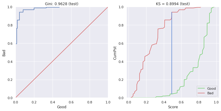
num = [ 'Sex', 'Pclass', 'Age', 'SibSp']

clf = pc.LogisticRegression(C = 0.5 ,penalty = 'l2')
clf.fit(train_features[num],train_labels)

score_l2 = clf.predict_proba(test_features[num])
mod_l2 = pc.ModelEval(score_l2[:,0], test_labels.values,'test')

mod_l2.ks_
ks:0.8994360902255639
print(clf_l2.intercept_,clf_l2.coef_)
[4.65600296] [[-2.6667898 -1.17940591 -0.34358811 -0.34700348]]
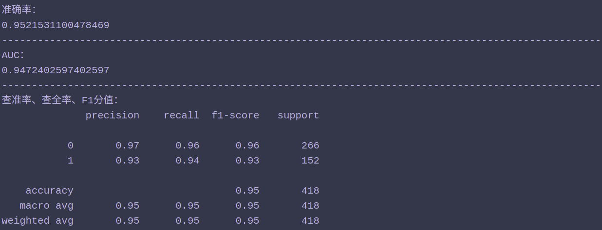
11、查看准确率、AUC、查准率、查全率以及F1-score
from sklearn.metrics import roc_auc_score
from sklearn.metrics import classification_report
from sklearn.metrics import accuracy_score
print('准确率:')
print(accuracy_score(test_labels.values ,clf_l2.predict(test_features[num])))
print('-'*100)
print('AUC:')
print(roc_auc_score(clf_l2.predict(test_features[num]), test_labels))
print('-'*100)
print("查准率、查全率、F1分值:")
print(classification_report(test_labels ,clf_l2.predict(test_features[num]) ,target_names=None))
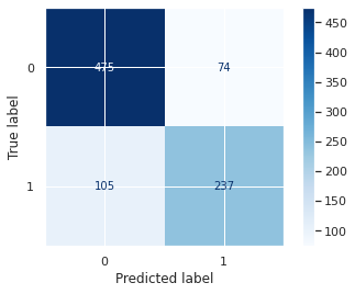
混淆矩阵:
from sklearn.metrics import plot_confusion_matrix
import matplotlib.pyplot as plt
plot_confusion_matrix(clf_l2 ,train_features[num] ,train_labels ,cmap=plt.cm.Blues)
plt.show()
12、最后还可以使用网格搜索进行参数调优,但是现在已经是最优的KS了,做了没有一点提升。
网格搜索代码:
from sklearn.model_selection import GridSearchCV
param_test1 ={'C':np.linspace(0.01,10,10000)}
gsearch1= GridSearchCV(
    estimator =pc.LogisticRegression(penalty='l2'),
        param_grid =param_test1,
        scoring='roc_auc',
        cv=5)
gsearch1.fit(train_features[num],train_labels)
一般情况logistic需要进行非常复杂的人工特征处理,所以在特征处理这个环节需要反复进行
logistic小结:
logistic回归是一种分类方法。
1、优点:
1、logistic回归模型直接对分类的可能性进行建模,无需事先假设数据满足某种分布类型。
2、logistic不仅可以预测样本类别,还可以得到预测为某类别的近似概率,这在许多需要利用概率辅助决策的任务中比较实用。
3、logistic使用的损失函数是任意阶可导的凸函数,有很好的数学性质,可避免局部最小值问题。
4、logistic对一般的分类问题都可以使用,特别是对稀疏高维特征的处理没有太大的压力,在处理类似广告点击率预测问题很有优势。
2、缺点:
1、logistic本质还是一种线性模型,只能做线性分类,不适合处理非线性问题,一般需要结合较多的人工特征处理使用。
2、logistic对正负样本的分布比较敏感,所以需要注意样本的平衡性。