pix2pix-tf官方文档

# 对抗网络的基本思想
# 假设有一种概率分布M，它相对于我们是一个黑盒子。为了了解这个黑盒子中的东西是什么，我们构建了两个东西G和D，
# G是另一种我们完全知道的概率分布，D用来区分一个事件是由黑盒子中那个不知道的东西产生的还是由我们自己设的G产生的。

# 不断的调整G和D，直到D不能把事件区分出来为止。在调整过程中，需要：
# 优化G，使它尽可能的让D混淆。
# 优化D，使它尽可能的能区分出假冒的东西。
# 当D无法区分出事件的来源的时候，可以认为，G和M是一样的。从而，我们就了解到了黑盒子中的东西。



from __future__ import absolute_import, division, print_function, unicode_literals

import tensorflow as tf

import os
import time
import random
import matplotlib.pyplot as plt
from IPython.display import clear_output


# 读取本地数据
PATH = os.path.join("/home/hxybs/facades/")


BUFFER_SIZE = 400
BATCH_SIZE = 1
#图片大小
IMG_WIDTH = 256
IMG_HEIGHT = 256


def load(image_file):
  image = tf.io.read_file(image_file)
  # 将JPEG编码图像解码为uint8张量
  image = tf.image.decode_jpeg(image)

  w = tf.shape(image)[1]

  w = w // 2
  # 图分两半，左边是真实的，右边是
  real_image = image[:, :w, :]
  input_image = image[:, w:, :]

  input_image = tf.cast(input_image, tf.float32)
  real_image = tf.cast(real_image, tf.float32)

  return input_image, real_image

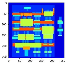
# 打开编号为100的jpg测试一下
inp, re = load(PATH+'train/100.jpg')
# 把草图和希望生成的图显示出来
plt.figure()
plt.imshow(inp/255.0)
plt.figure()
plt.imshow(re/255.0)

<matplotlib.image.AxesImage at 0x7ff77c4eb7b8>

def resize(input_image, real_image, height, width):
  # 调整大小，使用邻居差值
  input_image = tf.image.resize(input_image, [height, width],
                                method=tf.image.ResizeMethod.NEAREST_NEIGHBOR)
  real_image = tf.image.resize(real_image, [height, width],
                               method=tf.image.ResizeMethod.NEAREST_NEIGHBOR)
  return input_image, real_image


def random_crop(input_image, real_image):
  # 将两个合并成一个
  stacked_image = tf.stack([input_image, real_image], axis=0)
  # 随机地将张量裁剪为给定的大小  
  cropped_image = tf.image.random_crop(
      stacked_image, size=[2, IMG_HEIGHT, IMG_WIDTH, 3])

  return cropped_image[0], cropped_image[1]

# 归一化处理 to [-1, 1]

def normalize(input_image, real_image):
  input_image = (input_image / 127.5) - 1
  real_image = (real_image / 127.5) - 1

  return input_image, real_image


@tf.function()
def random_jitter(input_image, real_image):
  # resizing to 286 x 286 x 3
  input_image, real_image = resize(input_image, real_image, 286, 286)

  # randomly cropping to 256 x 256 x 3
  input_image, real_image = random_crop(input_image, real_image)

  if tf.random.uniform(()) > 0.5:
    # random mirroring
    input_image = tf.image.flip_left_right(input_image)
    real_image = tf.image.flip_left_right(real_image)

  return input_image, real_image


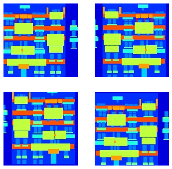
# 将图像进行随机变换：
# 1.将图像调整为更大的高度和宽度
# 2.随机裁剪为原始大小
# 3.随机水平翻转图像

# 显示随机变化后的图
plt.figure(figsize=(6, 6))
for i in range(4):
  rj_inp, rj_re = random_jitter(inp, re)
  plt.subplot(2, 2, i+1)
  plt.imshow(rj_inp/255.0)
  plt.axis('off')
plt.show()

# 加载训练数据
def load_image_train(image_file):
  input_image, real_image = load(image_file)
  input_image, real_image = random_jitter(input_image, real_image)
  input_image, real_image = normalize(input_image, real_image)

  return input_image, real_image

# 加载测试数据
def load_image_test(image_file):
  input_image, real_image = load(image_file)
  input_image, real_image = resize(input_image, real_image,
                                   IMG_HEIGHT, IMG_WIDTH)
  input_image, real_image = normalize(input_image, real_image)

  return input_image, real_image

# 读取数据
train_dataset = tf.data.Dataset.list_files(PATH+'train/*.jpg')
train_dataset = train_dataset.map(load_image_train,
                                   num_parallel_calls=tf.data.experimental.AUTOTUNE)
train_dataset = train_dataset.shuffle(BUFFER_SIZE)
train_dataset = train_dataset.batch(1)

test_dataset = tf.data.Dataset.list_files(PATH+'test/*.jpg')
test_dataset = test_dataset.map(load_image_test)
test_dataset = test_dataset.batch(1)

# 构造器的体系结构是经过修改的U-Net,由一个编码器（下采样器（downsampler））和一个解码器（上采样器（upsampler））组成。
# 编码器的构成（Conv2d-> Batchnorm-> LeakyReLU）
# 解码器的构成（Conv2DTranspose-> Batchnorm->Dropout（适用于前3个块）-> ReLU）
# 编码器和解码器之间存在跳跃连接。

# 输出信道数量为 3 是因为每个像素有三种可能的标签。把这想象成一个多类别分类，每个像素都将被分到三个类别当中。
OUTPUT_CHANNELS = 3

# 编码器
def downsample(filters, size, apply_batchnorm=True):
  initializer = tf.random_normal_initializer(0., 0.02)

  result = tf.keras.Sequential()
  result.add(
      tf.keras.layers.Conv2D(filters, size, strides=2, padding='same',
                             kernel_initializer=initializer, use_bias=False))
  if apply_batchnorm:
    result.add(tf.keras.layers.BatchNormalization())
  result.add(tf.keras.layers.LeakyReLU())

  return result

down_model = downsample(3, 4)
down_result = down_model(tf.expand_dims(inp, 0))
print (down_result.shape)

# 解码器
def upsample(filters, size, apply_dropout=False):
  initializer = tf.random_normal_initializer(0., 0.02)

  result = tf.keras.Sequential()
  result.add(
    tf.keras.layers.Conv2DTranspose(filters, size, strides=2,
                                    padding='same',
                                    kernel_initializer=initializer,
                                    use_bias=False))
  result.add(tf.keras.layers.BatchNormalization())
  if apply_dropout:
      result.add(tf.keras.layers.Dropout(0.5))
  result.add(tf.keras.layers.ReLU())

  return result

up_model = upsample(3, 4)
up_result = up_model(down_result)
print (up_result.shape)

(1, 128, 128, 3)
(1, 256, 256, 3)

# 构造器
def Generator():
  down_stack = [
    downsample(64, 4, apply_batchnorm=False), # (bs, 128, 128, 64)
    downsample(128, 4), # (bs, 64, 64, 128)
    downsample(256, 4), # (bs, 32, 32, 256)
    downsample(512, 4), # (bs, 16, 16, 512)
    downsample(512, 4), # (bs, 8, 8, 512)
    downsample(512, 4), # (bs, 4, 4, 512)
    downsample(512, 4), # (bs, 2, 2, 512)
    downsample(512, 4), # (bs, 1, 1, 512)
  ]

  up_stack = [
    upsample(512, 4, apply_dropout=True), # (bs, 2, 2, 1024)
    upsample(512, 4, apply_dropout=True), # (bs, 4, 4, 1024)
    upsample(512, 4, apply_dropout=True), # (bs, 8, 8, 1024)
    upsample(512, 4), # (bs, 16, 16, 1024)
    upsample(256, 4), # (bs, 32, 32, 512)
    upsample(128, 4), # (bs, 64, 64, 256)
    upsample(64, 4), # (bs, 128, 128, 128)
  ]

  initializer = tf.random_normal_initializer(0., 0.02)
  # 转置的2D卷积层
  last = tf.keras.layers.Conv2DTranspose(OUTPUT_CHANNELS, 4,
                                         strides=2,
                                         padding='same',
                                         kernel_initializer=initializer,
                                         activation='tanh') # (bs, 256, 256, 3)

  concat = tf.keras.layers.Concatenate()

  inputs = tf.keras.layers.Input(shape=[None,None,3])
  x = inputs

  # 在模型中降频取样
  skips = []
  for down in down_stack:
    x = down(x)
    skips.append(x)

  skips = reversed(skips[:-1])

  # 升频取样然后建立跳跃连接
  for up, skip in zip(up_stack, skips):
    x = up(x)
    x = concat([x, skip])

  x = last(x)

  return tf.keras.Model(inputs=inputs, outputs=x)

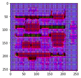
generator = Generator()

gen_output = generator(inp[tf.newaxis,...], training=False)
plt.imshow(gen_output[0,...])

Clipping input data to the valid range for imshow with RGB data ([0..1] for floats or [0..255] for integers).





<matplotlib.image.AxesImage at 0x7ff6bc7757f0>

# 鉴别器：PatchGAN。
# 鉴别器的构成（Conv-> BatchNorm-> Leaky ReLU）
# 最后一层之后的输出形状为（batch_size，30，30，1）
# 输出的每个30x30色块将输入图像的70x70部分分类（这种架构称为PatchGAN）。
# 鉴别器接收2个输入。
# 输入图像和目标图像，应将其分类为真实图像。
# 输入图像和生成的图像（生成器的输出），应将其分类为伪造的。
# 我们在代码中将这2个输入连接在一起（tf.concat（[inp，tar]，axis = -1））

def Discriminator():
  initializer = tf.random_normal_initializer(0., 0.02)

  inp = tf.keras.layers.Input(shape=[None, None, 3], name='input_image')
  tar = tf.keras.layers.Input(shape=[None, None, 3], name='target_image')

  x = tf.keras.layers.concatenate([inp, tar]) # (bs, 256, 256, channels*2)

  down1 = downsample(64, 4, False)(x) # (bs, 128, 128, 64)
  down2 = downsample(128, 4)(down1) # (bs, 64, 64, 128)
  down3 = downsample(256, 4)(down2) # (bs, 32, 32, 256)

  zero_pad1 = tf.keras.layers.ZeroPadding2D()(down3) # (bs, 34, 34, 256)
  conv = tf.keras.layers.Conv2D(512, 4, strides=1,
                                kernel_initializer=initializer,
                                use_bias=False)(zero_pad1) # (bs, 31, 31, 512)

  batchnorm1 = tf.keras.layers.BatchNormalization()(conv)

  leaky_relu = tf.keras.layers.LeakyReLU()(batchnorm1)

  zero_pad2 = tf.keras.layers.ZeroPadding2D()(leaky_relu) # (bs, 33, 33, 512)

  last = tf.keras.layers.Conv2D(1, 4, strides=1,
                                kernel_initializer=initializer)(zero_pad2) # (bs, 30, 30, 1)

  return tf.keras.Model(inputs=[inp, tar], outputs=last)

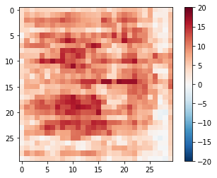
discriminator = Discriminator()
disc_out = discriminator([inp[tf.newaxis,...], gen_output], training=False)
plt.imshow(disc_out[0,...,-1], vmin=-20, vmax=20, cmap='RdBu_r')
plt.colorbar()

<matplotlib.colorbar.Colorbar at 0x7ff6bc495128>

# 定义 loss functions and the optimizer
# loss 由L1和cGAN组成

LAMBDA = 100

loss_object = tf.keras.losses.BinaryCrossentropy(from_logits=True)

def discriminator_loss(disc_real_output, disc_generated_output):
  real_loss = loss_object(tf.ones_like(disc_real_output), disc_real_output)

  generated_loss = loss_object(tf.zeros_like(disc_generated_output), disc_generated_output)

  total_disc_loss = real_loss + generated_loss

  return total_disc_loss

def generator_loss(disc_generated_output, gen_output, target):
  gan_loss = loss_object(tf.ones_like(disc_generated_output), disc_generated_output)

  # mean absolute error
  l1_loss = tf.reduce_mean(tf.abs(target - gen_output))

  total_gen_loss = gan_loss + (LAMBDA * l1_loss)

  return total_gen_loss

generator_optimizer = tf.keras.optimizers.Adam(2e-4, beta_1=0.5)
discriminator_optimizer = tf.keras.optimizers.Adam(2e-4, beta_1=0.5)

checkpoint_dir = './training_checkpoints'
checkpoint_prefix = os.path.join(checkpoint_dir, "ckpt")
checkpoint = tf.train.Checkpoint(generator_optimizer=generator_optimizer,
                                 discriminator_optimizer=discriminator_optimizer,
                                 generator=generator,
                                 discriminator=discriminator)

# 开始训练

EPOCHS = 20
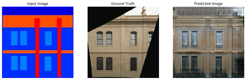
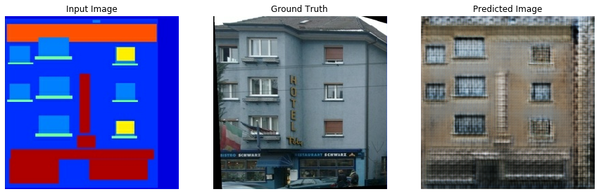
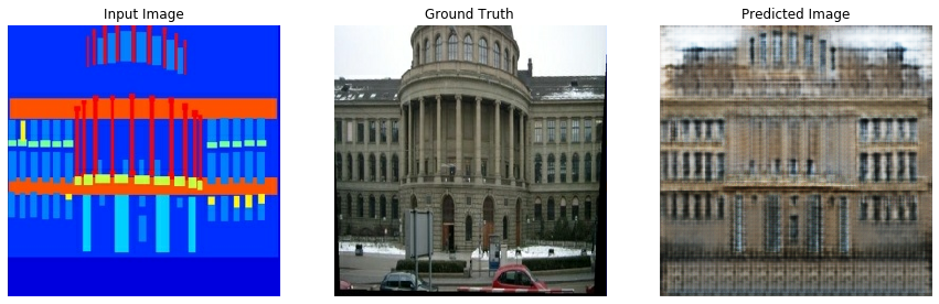
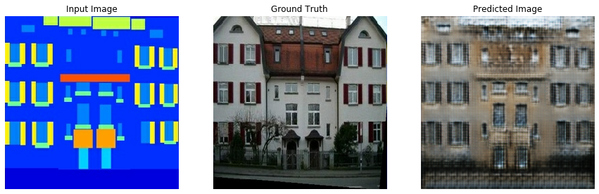
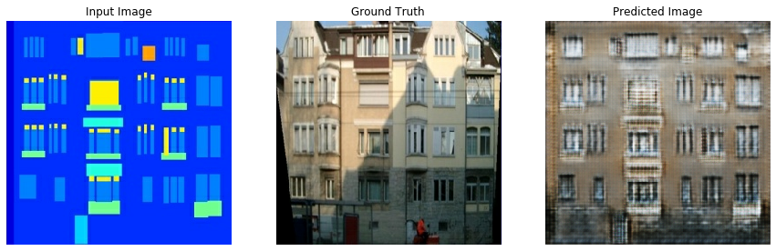
def generate_images(model, test_input, tar):
  # the training=True is intentional here since
  # we want the batch statistics while running the model
  # on the test dataset. If we use training=False, we will get
  # the accumulated statistics learned from the training dataset
  # (which we don't want)
  prediction = model(test_input, training=True)
  plt.figure(figsize=(15,15))

  display_list = [test_input[0], tar[0], prediction[0]]
  title = ['Input Image', 'Ground Truth', 'Predicted Image']

  for i in range(3):
    plt.subplot(1, 3, i+1)
    plt.title(title[i])
    # getting the pixel values between [0, 1] to plot it.
    plt.imshow(display_list[i] * 0.5 + 0.5)
    plt.axis('off')
  plt.show()

@tf.function
def train_step(input_image, target):
  with tf.GradientTape() as gen_tape, tf.GradientTape() as disc_tape:
    gen_output = generator(input_image, training=True)

    disc_real_output = discriminator([input_image, target], training=True)
    disc_generated_output = discriminator([input_image, gen_output], training=True)

    gen_loss = generator_loss(disc_generated_output, gen_output, target)
    disc_loss = discriminator_loss(disc_real_output, disc_generated_output)

  generator_gradients = gen_tape.gradient(gen_loss,
                                          generator.trainable_variables)
  discriminator_gradients = disc_tape.gradient(disc_loss,
                                               discriminator.trainable_variables)

  generator_optimizer.apply_gradients(zip(generator_gradients,
                                          generator.trainable_variables))
  discriminator_optimizer.apply_gradients(zip(discriminator_gradients,
                                              discriminator.trainable_variables))

def fit(train_ds, epochs, test_ds):
  for epoch in range(epochs):
    start = time.time()

    # Train
    for input_image, target in train_ds:
      train_step(input_image, target)

    clear_output(wait=True)
    # Test on the same image so that the progress of the model can be 
    # easily seen.
    for example_input, example_target in test_ds.take(1):
      generate_images(generator, example_input, example_target)

    # 保存 (checkpoint) 每 20 epochs
    if (epoch + 1) % 20 == 0:
      checkpoint.save(file_prefix = checkpoint_prefix)

    print ('Time taken for epoch {} is {} sec
'.format(epoch + 1, time.time()-start))
fit(train_dataset, EPOCHS, test_dataset)

Time taken for epoch 20 is 203.97532176971436 sec

checkpoint.restore(tf.train.latest_checkpoint(checkpoint_dir))
# Run the trained model on the entire test dataset
for inp, tar in test_dataset.take(5):
  generate_images(generator, inp, tar)